
Modeling Pinhole Phenomenon in Sanitary Porcelains Case Study: Isatis Sanitary Porcelain Plant, Yazd, Iran
- DOI
- 10.2991/jsta.2018.17.3.11How to use a DOI?
- Keywords
- sanitary porcelain; pinhole; artificial neural networks; regression; correlation coefficient
- Abstract
Sanitary porcelain products might have several defects, causing potential high-grade desirable products be converted into low-grade ones. Some of the defects are such that a few of them in the products will result in a great fall of product rating and consequently reduction of its value and price. Among these defects is a defect called pinhole. In this article, it has been tried to identify, from a list of factors, the most influential factors of the production process which cause the pinhole defect affecting the product rating. It then tries to present a prediction model for the number of pinholes. For this purpose, initially seven factors were chosen to help presenting a suitable prediction model and several statistical tools and artificial intelligence prediction tools were investigated to present a suitable prediction model. The presented model could be used by the company to enhance the product rating through choosing right value for the right factors causing the pinhole defect and to decrease the wastes and the expenditures.
- Copyright
- © 2018, the Authors. Published by Atlantis Press.
- Open Access
- This is an open access article under the CC BY-NC license (http://creativecommons.org/licences/by-nc/4.0/).
1. Introduction
Defects in sanitary-ware products affect the quality (rating) of the products and the factory expenditures. If we can predict the defects through a model, we would be able to predict the rating, to enhance the quality and to reduce the wastes and expenditures, by choosing right amounts for the factors participating in the model. Several defects (blisters, pinholes, specks, stuck, cracks, deformation, green spots,...) may be found in sanitary porcelains which tend to reduce the rating of these products. Some of these defects are identified before the baking phase and some are identified after the phase. The defective products with defects identifiable after the baking phase are not suitable for reproduction pinholes, which are quality flaw appearing as small holes in the fired glaze surface, are among the defects which could be identified after baking phase.
This defect might occur on all part of the surface of sanitary-ware products. Figure 1 shows a surface having this flaw. A survey performed in Isatis sanitary porcelain manufacturing co., Yazd, Iran shows that 10.5% of the defective products is due to ’pinhole’ flaw and causes severe losses to the manufacturer; due to this reason the manufacturer decided to do a research on pinhole[1]. The present article is based on the research. The manufacturing company would like to know if there is a relationship between "the number of pinholes in the products" and some factors such as the followings:
Glaze viscosity(V)
Surface tension of raw material(ST)
Speed of reaching the maximum temperature(SMT)
Glaze cooling speed(SC)
The maximum temperature of the furnace (MT)
Abrasion of Glaze raw materials(AG)
glaze dying time(TD)
curvature(S=smooth or C =curved)
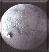
Pinholes in a sanitary-ware product
The purpose of the present research is to find the key factors (if any) causing the pinhole phenomena from the above list and, using the key factors as input, to present a model for predicting the number pinholes in the product and thereby predicting the rating of the products with pinholes. If a suitable model is reached, the quality of the products could be improved by modifying the factors and the plant expenditures be decreased. This research is based on [1] and our literature survey did not result in any significant work in the prediction of pinhole defect; therefore this research could be regarded a new one. However [2] and [3] are helpful references for understanding some concepts regarding ceramics and component analysis used in this research.
2. Data
The data for this research is obtained from producing 42 curved and 122 smooth specimens with dimension of nearly 10cm × 10cm at Istatis sanitary-ware plant located in Yazd, Iran with different values for V, ST, SMT, MT, AG & TD. Table 1 shows the mean of the values used for V, ST, SMT, MT, AG & TD variables and the mean number of pinholes created in 164 specimen as well as some other information (minimum, maximum, median, range, standard deviation) about the mentioned features.
| Feature (dimension) | Curvature | Mean | Median | Minimum | Maximum | Range | Std. Dev. |
|---|---|---|---|---|---|---|---|
| V (poise) | S | 138.459 | 137.00 | 111.00 | 181.00 | 80.000 | 16.965 |
| C | 139.357 | 139.00 | 111.50 | 191.00 | 89.500 | 24.697 | |
| ALL | 138.689 | 137.50 | 111.00 | 191.00 | 90.000 | 19.163 | |
| ST (G) | S | 4.558 | 4.575 | 3.33000 | 5.680 | 2.350 | 0.396 |
| C | 4.784 | 4.825 | 2.79000 | 6.840 | 4.050 | 0.877 | |
| ALL | 4.616 | 4.605 | 2.79000 | 6.840 | 4.050 | 0.565 | |
| SMT (minute) | S | 312.746 | 312.80 | 309.00 | 315.800 | 6.800 | 1.250 |
| C | 313.371 | 313.25 | 307.70 | 318.800 | 11.10 | 2.250 | |
| ALL | 312.906 | 312.90 | 307.70 | 308.800 | 1.10 | 1.584 | |
| SC (minute) | S | 438.302 | 438.40 | 428.00 | 447.000 | 19.00 | 3.108 |
| C | 439.867 | 439.45 | 424.100 | 453.000 | 29.90 | 5.994 | |
| ALL | 438.703 | 438.65 | 424.100 | 453.000 | 29.90 | 4.084 | |
| MT (centigrade) | S | 1084.468 | 1085.45 | 1061.100 | 1094.000 | 33 | 6.416 |
| C | 1084.160 | 1083.50 | 1064.20 | 1109.000 | 45 | 8.681 | |
| ALL | 1084.389 | 1084.800 | 1061.10 | 1109.000 | 48 | 7.038 | |
| AG (mesh) | S | 2.80 | 2.87 | 1.84 | 3.16 | 1.32 | 2.633 |
| C | 2.81 | 2.80 | 2.02 | 3.69 | 1.67 | 3.09 | |
| ALL | 2.80 | 02.84 | 1.84 | 3.69 | 1.85 | 2.74 | |
| TD (second) | S | 133.211 | 133.300 | 130.20 | 135.90 | 5.700 | 1.906 |
| C | 133.479 | 133.550 | 131.40 | 135.40 | 4.00 | 1.89 | |
| ALL | 133.280 | 133.350 | 130.20 | 135.90 | 5.70 | 1.90 | |
| Pinhole | S | 7.21 | 4.46 | 0 | 40 | 40 | 7.62 |
| C | 10.55 | 7.16 | 1 | 29 | 28 | 7.63 | |
| ALL | 8.87 | 5.97 | 0 | 40 | 40 | 7.69 | |
mean, median, minimum, maximum, range, standard deviation of the initial data
2.1 Initial evaluation of data
Figure 2 shows the probability plot the number of pinholes in both curved (C) and smooth (S) specimens. According to the figure the pinhole data are not normally distributed.
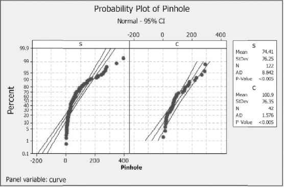
Normal probability plot for the pinholes in the sample
An algorithm called Johnson transformation was applied on the pinhole data. The resulted data is referred as J-pinhole. As the normal probability plot of J-pinhole in Fig. 3 shows, the J-pinhole data is normally distributed.
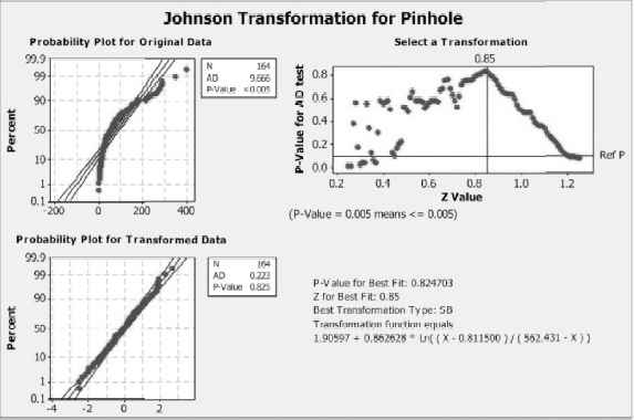
Normal probability plot for J-pinhole data (i.e. the number of inholes in the specimens after applying Johnson transformation)
A fit of linear regression model including all variables i.e. V, ST, SMT, MT, AG, TD to predict number of pinholes showed that the model is not appropriate for the pinhole data.
A stepwise regression model was then applied to J-pinhole data. Table 2 shows the result. The model correlation coefficient was 11% which is not acceptable.
| Alpha-to-Enter: 0.15 Alpha-to-Remove: 0.15 | |||||
| Response is J_Pinhole on 8 predictors, with N = 164 | |||||
| Step | 1 | 2 | |||
| Constant | −0.1354 | −2.1142 | SMT | 0.148 | |
| V | 0.0113 | 0.0113 | T-Value | 3.08 | |
| T-Value | 2.82 | 2.90 | P-Value | 0.002 | |
| P-Value | 0.005 | 0.004 | S | 0.981 | 0.957 |
| CURVE- | −0.42 | −0.33 | R-Sq | 7.97 | 13.12 |
| T-Value | −2.39 | −1.89 | R-Sq(adj) | 6.83 | 11.50 |
| P-Value | 0.018 | 0.061 | Mallows Cp | 16.1 | 8.4 |
Stepwise Regression: J_Pinhole versus V, ST,
These two experiments indicate either the relationship between pinhole data as the response versus V, ST, SMT,…. is not linear or some other variables should be considered or stronger tools are needed to model the relationship.
In the rest of this research J-pinhole data which are normally distributed are used.
What follows is about the effect of curvature on the number of pinholes.
The relationship between curvature and pinholes
To study the effect of curvature on the number of pinholes the following 2 tests of hypothesis were performed on the smooth and curved specimens:
- A)
a two sided F-test for the equality of the variance of J-pinhole data concerning curved surface and the variance of J-pinhole data concerning smooth surface;
- B)
a two sided t-test for the equality of the mean of J-pinhole data concerning curved surface and the mean of J-pinhole data concerning smooth surface.
We were allowed to perform the F-test & t-test on the J-pinholes data, because these data were proved to be normally distributed. Tables 3 &4 shows the results
| A) Test and CI for Two Variances: J_Pinhole vs Curve | ||||||
|---|---|---|---|---|---|---|
| Method | ||||||
| Null hypothesis | Sigma(S) / Sigma(C) = 1 | |||||
| Alternative hypothesis | Sigma(S) / Sigma(C) not = 1 | |||||
| Significance level | Alpha = 0.05 | |||||
| 95% Confidence Intervals CI for | ||||||
| Statistics curve | N | St. Dev | Variance | Distribution of Data | CI for StDe Ratio | Variance Ratio |
| s | 122 | 1.021 | 1.043 | Normal | (0.827, 1.372) | (0.684, 1.882) |
| c | 42 | 0.944 | 0.891 | Continuous | (0.833, 1.492) | (0.695, 2.227) |
| Ratio of standard deviations = 1.082 | ||||||
| Ratio of variances = 1.171 | ||||||
|
|
||||||
| Tests | ||||||
| Test Method | DF1 | DF2 | Statistic | P-Value | ||
| F Test (normal) | 121 | 41 | 1.17 | 0.571 | ||
| Levene’s Test (any continuous) | 1 | 162 | 0.72 | 0.397 | ||
F-test for the equality of variances of J_Pinholes in the smoothed and curved surfaces
| B) Two-Sample t-test and CI: J_Pinhole, curvature | ||||
|---|---|---|---|---|
| Cur. | N | Mean | St Dev | SE Mean |
| s | 122 | −0.12 | 1.02 | 0.092 |
| c | 42 | 0.310 | 0.944 | 0.15 |
| Difference = mu (s) − mu (c) | ||||
| Estimate for difference: −0.431 | ||||
| 95% CI for difference: (−0.785, −0.076) | ||||
| T-Test of difference = 0 (vs not =): T-Value = −2.40 P-Value = 0.017 DF = 162 | ||||
| Both use Pooled StDev = 1.0023 | ||||
t-test for the equality of mean of J_Pinholes in the smoothed and curved surfaces
From Table 3 it could be concluded that curvature does not increase or decrease the variance of the number of pinholes.
The t-test of Table 4 indicate that, on the average, the surface curvature causes more pinholes in comparison to the surface smoothness.
Are variables V, ST, SMT, MT, AG, TD normally distributed ?
Utilizing Anderson-Darling test show that some of the variables are normally distributed and some not. The result of the test for both curved and smooth cases is shown in Table 5.
| Feature | V | ST | SMT | SC | MT | AG | TD |
|---|---|---|---|---|---|---|---|
| smooth | ☑ | ☑ | ☑ | ☑ | - | - | - |
| curved | ☑ | ☑ | ☑ | ☑ | - | - | ☑ |
The status of the normality of the distribution of variables
As Table 5 indicates the variables MT, AG are not normally distributed for both cases (smooth& curved) and TD is not normally distributed for smooth case. As stated earlier, J-pinhole data i.e. the results of Johnson transformation on the pinhole data will be used throughout this research.
3. Description of the method
The steps carried out during our research is as follows:
3.1. Step 1: Evaluation of data-detection of outlier data
In this phase of step 1 the outliers are detected in the multivariate data. Pair-wise scatter plots will not work as it is possible for an outlier to exist in all dimensions but not an outlier in any of the 2 dimensional subspaces.
It is important to realize, cases which are multivariate outliers may not necessarily be univariate outliers. In other words being an outlier on one of the variables under consideration is not necessarily a multivariate outlier.
One of the best ways to check for multivariate outliers is through Mahalanobis’ distance. Mahalanobis’ distance accounts for the different scale and the variance of each of the variables in a probabilistic way; in other words, if one considers the probability of a case being a member of the multivariate distribution, then one must account for the density function, or standard deviation, of each variable in the multivariate set. Minitab 16 which does such a multivariate outliers detection resulted in Fig. 4.
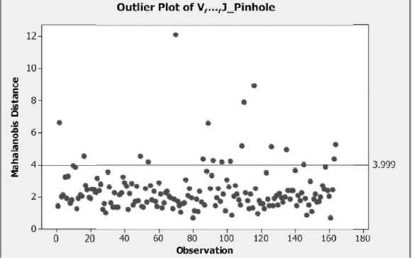
Mahalanobis interval for the factors causing pinhole defect
One smooth specimen which had too much Mahalanobis’ distance was excluded from 164 (122 smooth +42 curved) pieces and Table 1 was updated into Table 6 according to the remaining 121 and 42 pieces.
| Feature (dimension) | Curve | Mean | Median | Minimum | Maximum | Range | Std. Dev. |
|---|---|---|---|---|---|---|---|
| V (poise) | S | 138.34 | 137.00 | 101.00 | 181.0000 | 80.00 | 16.99 |
| C | 139.35 | 139.00 | 101.500 | 191.0000 | 89.50 | 24.69 | |
| ALL | 138.60 | 137.00 | 101.000 | 191.0000 | 90.00 | 19.19 | |
| ST (G) | S | 4.55 | 4.57 | 3.3300 | 5.6800 | 2.35 | 0.39443 |
| C | 4.78 | 4.82 | 2.790 | 6.8400 | 4.05 | 0.87 | |
| ALL | 4.61 | 4.60 | 2.790 | 6.8400 | 4.05 | 0.56 | |
| SMT (minute) | S | 312.72 | 312.80 | 309.00 | 315.8000 | 6.80 | 1.23 |
| C | 313.37 | 313.25 | 307.70 | 318.8000 | 11.10 | 12.25 | |
| ALL | 312.89 | 312.90 | 307.70 | 318.8000 | 11.10 | 11.58 | |
| SC (minute) | S | 438.30 | 438.40 | 428.00 | 447.0000 | 19.00 | 13.12 |
| C | 439.86 | 439.45 | 424.10 | 453.0000 | 28.90 | 15.99 | |
| ALL | 438.70 | 438.70 | 424.10 | 453.0000 | 28.90 | 14.09 | |
| MT (centigrade) | S | 1084.46 | 1085.50 | 1061.10 | 1094.0000 | 32.90 | 6.44 |
| C | 1084.15 | 1083.50 | 1064.20 | 1109.0000 | 44.80 | 8.68 | |
| ALL | 1084.38 | 1084.80 | 1061.10 | 1109.0000 | 47.90 | 7.05 | |
| AG (mesh) | S | 2.80 | 2.87 | 1.84 | 3.16 | 1.32 | 0.26 |
| C | 2.81 | 2.80 | 2.02 | 3.69 | 1.67 | 0.30 | |
| ALL | 2.80 | 2.84 | 1.84 | 3.69 | 1.85 | 0.27 | |
| TD (second) | S | 133.20 | 133.30 | 130.20 | 135.90 | 5.70 | 1.90 |
| C | 133.47 | 133.55 | 131.40 | 135.40 | 4.0 | 1.89 | |
| ALL | 133.27 | 133.30 | 130.20 | 135.90 | 5.70 | 1.90 | |
| Pinhole | S | 7.47 | 5.10 | 4 | 40 | 36 | 7.64 |
| C | 10.08 | 7.80 | 4 | 29 | 25 | 7.63 | |
| ALL | 8.144 | 5.80 | 4 | 40 | 36 | 7.70 | |
(revised Table 1) Data for model development
3.1.1 The relationship between variables V, ST, SMT, MT, AG, TD and J-pinhole
The scatter plot of J-pinhole versus individual variables as well as scatter plot of every pair of variables are given in the matrix plot shown in Fig. 5. The red cycle have been used for curved specimens and the black cycle for smooth specimens
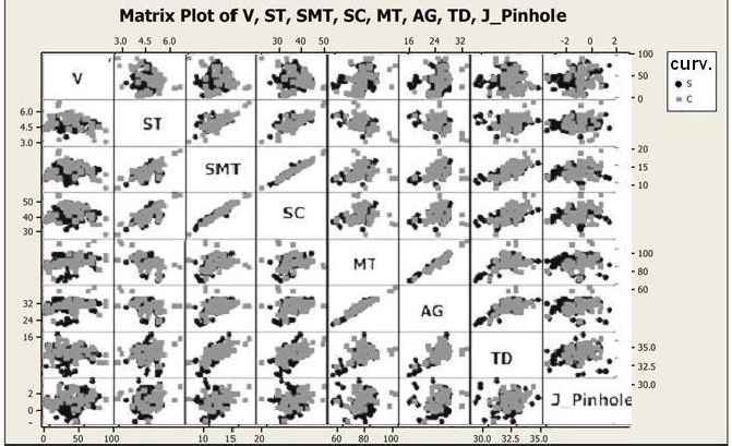
Matrix plot of V, ST, SMT, SC, MT, AG, TD and J-pinhole
As Fig. 5 shows AG & MT, and also SC&SMT are strongly linearly correlated.
Table 7 shows the correlation coefficient ( R) between the J-pinhole and individual variables as well as between each pair of the variables, calculated using SPSS software.
| Correlations | V | ST | SMT | SC | MT | AG | TD |
|---|---|---|---|---|---|---|---|
| ST | −0.176 | ||||||
| SMT | −0.004 | 0.666 | |||||
| SC | −0.001 | 0.733 | 0.983 | ||||
| MT | 0.263 | −0.549 | 0.227 | 0.153 | |||
| AG | 0.219 | −0.43 | 0.376 | 0.274 | 0.97 | ||
| TD | 0.004 | 0.109 | 0.667 | 0.523 | 0.462 | 0.658 | |
| J-Pinhole | 0.219 | 0.168 | 0.26 | 0.251 | 0.09 | 0.135 | 0.178 |
Correlation coefficients(R)
3.1.2 Problem Dimension reduction
As the last row of Table 7 shows, J-pinhole has the greatest correlation with SMT and the least correlation with MT. There are several filtering (feature selection) approaches to removing irrelevant data, eliminating redundant features from a set of features and reducing the number of features or variables. Correlation-based Feature Selection (CFS), Principal Component Analysis (PCA), Fast Correlation based Feature selection , Gain Ratio Attribute Evaluation, Chi-square Feature Selection, Fast Information-Gain-Ratio Feature selection, and Markov Blanket Filter are among the feature selection techniques proposed by researchers for feature selection. In this research, CFS and PCA were utilized for finding the principal components of data and reducing the problem dimension.
Some softwares such as MINITAB have the capability of reducing the number of variables of the problem utilizing Principal component analysis (PCA ) tool. For the variables causing pinhole defect, MINITAB was used to do the analysis. Table 8 shows the result of the analysis.
| Principal Component Analysis on Factors : V, ST, SMT, SC, MT, AG, TD Eigen analysis of the Correlation Matrix |
|||||||
|---|---|---|---|---|---|---|---|
| Eigenvalue | 3.1892 | 2.4881 | 0.9361 | 0.3745 | 0.0095 | 0.0022 | 0.0005 |
| Proportion | 0.456 | 0.355 | 0.134 | 0.053 | 0.001 | 0.000 | 0.000 |
| Cumulative | 0.456 | 0.811 | 0.945 | 0.998 | 1.000 | 1.000 | 1.000 |
| Variable | PC1 | PC2 | PC3 | PC4 | PC5 | PC6 | PC7 |
| V | 0.066 | 0.221 | −0.953 | 0.197 | −0.001 | −0.005 | −0.000 |
| ST | 0.166 | −0.598 | −0.134 | −0.034 | −0.762 | 0.124 | 0.016 |
| SMT | 0.507 | −0.263 | −0.046 | 0.106 | −0.279 | −0.404 | 0.647 |
| SC | 0.469 | −0.316 | −0.109 | −0.322 | 0.412 | 0.252 | −0.576 |
| MT | 0.330 | 0.487 | 0.051 | −0.398 | −0.199 | 0.587 | 0.330 |
| AG | 0.406 | 0.428 | 0.104 | −0.130 | −0.364 | −0.594 | −0.372 |
| TD | 0.466 | 0.068 | 0.216 | 0.818 | 0.013 | 0.245 | −0.040 |
Principal component analysis (PCA)
The first 4 variables i.e. V, ST, SMT, SC were selected using PCA.
The data of V, ST, SMT, SC as well as curvature and J-pinhole data are identified as “PCA data set”.
Some softwares, such as WEKA, do CFS study to reduce a problem dimension. Table 9 shows the result of applying this study on our problem.
| === Run information === Evaluator: weka.attributeSelection.CfsSubsetEval Search: weka.attributeSelection.BestFirst -D 1 -N 5 Relation: FINAL-weka.filters.unsupervised.attribute.Remove-R9–10 Instances: 163 Attributes: 9 V Curve ST SMT SC MT AG TD J_Pinhole Evaluation mode: evaluate on all training data |
>>>>>>>> === Attribute Selection on all input data === Search Method: Best first. Start set: no attributes Search direction: forward Stale search after 5 node expansions Total number of subsets evaluated: 39 Merit of best subset found: 0.287 Attribute Subset Evaluator (supervised, Class (numeric): 9 J_Pinhole): CFS Subset Evaluator Including locally predictive attributes Selected attributes: 1,2,4 : 3 V Curve SMT |
A correlation-based feature selection (CFS)) on factors causing pinholes
This CFS study selects variables V, SMT as well as curvature as the principal characteristics causing pinhole flaw in the products of Isatis sanitary-ware plant. V, SMT as well as curvature and J-pinhole data are identified as “CFS data set”.
3.2 Step 2: Data pre-processing
The other variables are modified according the following relationship:
3.3 Step 3: Choosing right variables for the regressors
In this research neural network and regression modeling are used to predict the number of pinholes in the products.
We have identified 3 sets of data so far Full set data including V, ST, SMT, SC, MT, AG, TD, curvature and J-pinhole, “PCA data set” and “CFS data set”. In step 3 we will try to find which set(s) should be chosen for modeling.
Using 3 sets of data, several multi-layer perception (MLP), Radial Basis Functions (RBF), generalized regression neural networks (GRNN) were trained as well as Additive Regression. The efficiency of the model was calculated using the mean squared error (MSE) and also correlation coefficient (R) of the observed set of data and the corresponding set predicted by the model. Table 10 shows the result.
| GRNN | MLP | RBF | Additive Regression | |||||
|---|---|---|---|---|---|---|---|---|
| Data set | MSE | R | MSE | R | MSE | R | MSE | R |
| Full | 0.80835 | 0.289185 | 1.165752 | 0.2344 | 1.055551 | 0.0402 | 1.006812 | 0.3343 |
| PCA | 0.78939 | 0.29601 | 0.041047 | 0.2586 | 0.037018 | 0.1412 | 0.043765 | 0.1737 |
| CFS | 0.52889 | 0.316223 | 1.12169281 | 0.205 | 1.061724 | 0.0308 | 0.975551 | 0.3262 |
Comparison of the efficiency of different models
Table 10 shows that the RBF neural networks used for the research produced poor correlation coefficient; therefore it was excluded.
Figure 6 shows the coefficient of variation between observed and predicted pinhole data using different regressor and different inputs. The PCA and CFS sets of data produced better results compared to the full set, as evident from MSE and R indices.
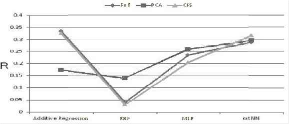
Correlation coefficient for different repressors using different inputs sets
More study lead to choosing MLP and GRNN networks as well as Additive Regression with the following inputs for entering the next step.
| regressor | Input data set |
|
|---|---|---|
| CFS | PCA | |
| MLP | ☒ | ☑ |
| Additive regression | ☑ | ☑ |
| GRNN | ☑ | ☒ |
Inputs suitable for the modeling tools
3.4 Step 4: Training
MATLAB was used to train GRN. MLP was trained with WEKA. Additive regression was applied by WEKA. To train the regressor networks each data set were divided into two subsets i.e. a subset for training and a subset for testing the regressor with the proportion of 2 to 1. The efficiency of the 3 modeling tools was determined by R and MSE as shown in Table 12 and figures 7&8.
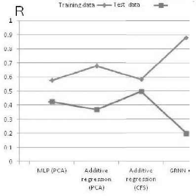
Correlation coefficient of observed and predicted data for different regressors
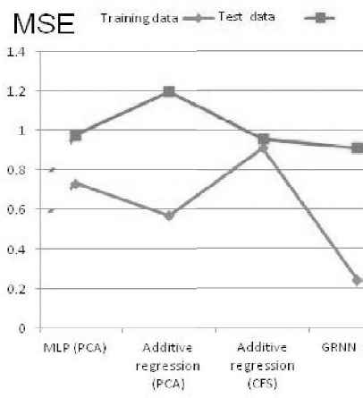
Mean squared error of observed and predicted data for different regressors
| MSE | R(%) | |||
|---|---|---|---|---|
| training | test | training | test | |
| MLP (PCA) | 0.731367 | 0.975946 | 57.68 | 42.47 |
| Additive regression (PCA) | 0.569119 | 1.197711 | 67.79 | 36.90 |
| Additive regression (CFS) | 0.912579 | 0.957601 | 58.49 | 0.49.75 |
| GRNN (CFS) | 0.246 | 0.9119 | 88 | 20 |
Efficiency of the 3 modeling tool
GRNN correlation coefficient for the training data is high, while this index for test data is low; which might be due to over-fitting. This inference could also be made from evaluating the MSE for the training and the test data sets. This observation lead in the exclusion of the GRNN network. Although one could make a similar argument for Additive Regression (with PCA data set as input); but we do not exclude it because the way it has dealt with the test data is not that different from the other methods.
3.5 Combination of the regressors
In this phase of step 4, the weighted average of the results of each two different regressors is calculated and the pair with the better R & MSE is determined. Various weights were tested. Figures 9 and 10 are the plots for showing how efficiency varies with the weight for one combination i.e. “MLP(PCA)+Additive Regression (PCA)” as an example.
The best MSE occurs at weight=0.28 for the training data and weight=0.76 for the data.
The best R occurs at weight=0.28 for the training data and weight=0.66 for the test data.
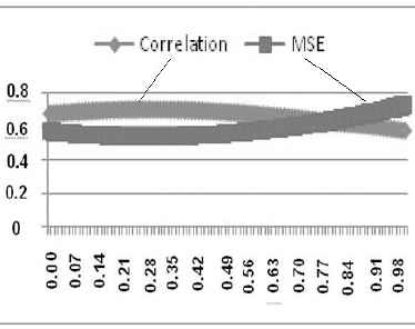
The efficiency versus weight for “MLP+Additive regression” (PCA)-training data
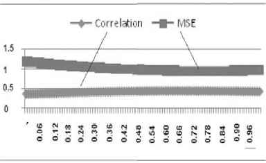
The efficiency versus weight for “MLP+Additive regression” (PCA)-test data
Table 13 shows the result of identifying the weights with the best efficiency based on R and MSE different combinations.
| R(%) | weight | MSE | weight | ||||||
|---|---|---|---|---|---|---|---|---|---|
| Combined regressors | training | test | training | test | training | test | training | test | |
| Additive Regression (PCA) | MLP (PCA) | 70.19 | 44.07 | 0.28 | 0.66 | 0.540745441 | 0.952535 | 0.28 | 0.76 |
| Additive Regression (CFS) | MLP (PCA) | 63.13 | 50.72 | 0.40 | 0.20 | 0.63486065 | 0.839146 | 0.44 | 0.07 |
| Additive Regression (CFS) | Additive Regression (PCA) | 70.14 | 47.26 | 0.64 | 0.55 | 0.55380549 | 0.795623 | 0.75 | 0.73 |
the weights in Table 13 corresponds to the regrressor colored in gray.
The efficiency of combined regressors*
Figure 11 compares R for the 3 combinations.
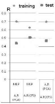
Correlation coefficient of the observed and predicted data for combination of regressors
Our criteria for choosing the suitable combination is having relative high efficiency based on R & MSE and the closeness of the R & MSE for training data set with those for the test data set. This lead us in choosing the combination of MLP and the additive regression with the input obtained from CFS analysis, which has the best results among the combinations.
Table 14 shows that the efficiency of the combination of the 2 regressors is better than the efficiency of the individuals.
| MSE | R (%) | |||
|---|---|---|---|---|
| training | test | training | test | |
| Additive regression (CFS) + MLP (PCA) | 0.63486065 | 0.839146 | 63.13 | 50.72 |
| MLP (PCA) | 0.731367 | 0.975946 | 57.68 | 42.47 |
| Additive regression (CFS) | 0.912579 | 0.957601 | 58.49 | 49.75 |
Comparison of the chosen combination and the components
According to the result of CFS analysis V, SMT as well as curvature have the most influence on the number of pinholes, and according to the PCA analysis V, ST, SMT, SC as well as curvature are the most influential variables.
Based on a sensitivity analysis SMT is the most influential variable affecting the number of pinholes.
Conclusions
This research shows that
- 1)
In the production process of sanitary-ware products at Isatis sanitary porcelain plant, Yazd, Iran , Glaze viscosity (V) and the speed of reaching the maximum temperature (SMT) as well as curvature (as opposed to smoothness of the product) and also the surface tension of raw material (ST)and glaze cooling speed (SC) are the most influential characteristics affecting the number of pinholes occurring in the finished product of the plant.
- 2)
Multilayer perception neural networks and additive regression proved to be efficient in predicting the number of pinholes and thereby the rating of the product. Trial and error with giving different values for the input variables of these models could yield a design the production design experiment which could result in low wastes and reduction of costs.
For future research, other factors (other than V, ST, SMT, MT, AG & TD as well as curvature) might be studied and other modeling tools such as other neural networks might be tested.
References
Cite this article
TY  - JOUR
AU  - H. Bazargan
AU  - A. Dehghanzadeh
PY  - 2018
DA  - 2018/09/30
TI  - Modeling Pinhole Phenomenon in Sanitary Porcelains Case Study: Isatis Sanitary Porcelain Plant, Yazd, Iran
JO  - Journal of Statistical Theory and Applications
SP  - 572
EP  - 586
VL  - 17
IS  - 3
SN  - 2214-1766
UR  - https://doi.org/10.2991/jsta.2018.17.3.11
DO  - 10.2991/jsta.2018.17.3.11
ID  - Bazargan2018
ER  -