
Estimating the Parameters of a Generalized Exponential Distribution
- DOI
- 10.2991/jsta.2018.17.3.9How to use a DOI?
- Keywords
- Generalized exponential distribution; Maximum Likelihood Estimation; Method of Moments; Moment generating function; Sufficient condition
- Abstract
A three-parameter generalized exponential distribution was suggested by Hossain and Ahsanullah [5]. Some important aspects of this distribution in the area of estimation remain unexplored in the earlier works. We discuss here the maximum likelihood (ML) method and the method of moments to estimate the parameters. The sufficient condition for the existence of a unique solution of the parameters obtained by the method of moments is derived. Finally, a popular real life numerical example is illustrated to investigate the application of both methods of estimation and the results obtained therein are compared with four similar well known three-parameter distributions.
- Copyright
- © 2018, the Authors. Published by Atlantis Press.
- Open Access
- This is an open access article under the CC BY-NC license (http://creativecommons.org/licences/by-nc/4.0/).
1. Introduction
The estimation of parameters and drawing conclusions based on the estimated parameters is one of the important aspects of inferential statistics. The three-parameter gamma and Weibull distributions are commonly used in life time data analysis. These distributions have many desirable statistical properties. For more information on these distributions see Alexander [1] and Jackson [6].
Mudholkar [9] considered a three-parameter exponentiated Weibull distribution. This new family is suitable for modeling data that indicate non-monotone hazard rates and can be adopted for testing goodness of fit of Weibull as a submodel. It is a right skewed unimodal density function. The usefulness and flexibility of the family is illustrated by reanalyzing five classical data sets on bus-motor failures.
Gupta [3] proposed special cases of the exponentiated Weibull and exponentiated exponential models and compared their performances with the two-parameter gamma family and two-parameter Weibull family, mainly through data analysis and computer simulations. For more on exponentiated Weibull, beta Gumbel, and beta exponentiated distribution see Nadarajah [10], Nadarajah and Kotz [11], Nadarajah and Kotz [12], Nassar and Eissa [13], and Raqab and Ahsanullah [14].
A three-parameter generalized exponential distribution was suggested by Gupta and Kundu [4]. This distribution is a particular case of the exponentiated Weibull distribution originally proposed by Mudholkar, Srivastava, and Freimer [9]. Since its distribution function has closed form the inference based on the censored data can be handled more easily than gamma family. One of its drawbacks being it is less flexible than the other two families for graduating tail thickness.
Recently, Kundu and Gupta [7] introduced the bivariate generalized exponential distribution so that the marginal have generalized exponential distributions. They reanalyzed one set of data and the results have shown that the bivariate generalized exponential distribution provides a better fit than the bivariate exponential distribution.
Hossain and Ahsanullah [5] introduced a new three-parameter generalized exponential distribution that represents a different type of generalization than Gupta and Kundu [4]. This distribution approaches a two parameter exponential distribution when the shape parameter approaches zero, whereas the distribution in Gupta and Kundu [4] approaches two-parameter exponential if the shape parameter approaches one.
In this article we have considered the estimation of parameters of the three-parameter generalized exponential distribution introduced by Hossain and Ahsanullah [5] by using the maximum likelihood estimation and the method of moments. A sufficient condition for the existence of unique solution for the parameters estimated by the method of moments is derived. A real time numerical example is analyzed and compared with four other similar distributions.
The rest of the article is organized as follows: Section 2 introduces the generalized exponential distribution and some its important properties. In section 3 we described the parameter estimation procedure using maximum likelihood method and method of moments. In section 4 we showed the applications by analyzing a set of real time data and compared the results with similar three-parameter distributions.
2. Generalized Exponential Distribution
2.1 Distribution and density functions
A random variable X is said to have generalized exponential distribution (GE2) if it has the following distribution function
The generalized exponential distribution introduced by Gupta and Kundu [4] is given by
To keep a clear distinction between GE2 and the Gupta and Kundu [4], the generalized exponential distribution in Gupta and Kundu [4] will be denoted as GE1.
The graphs of probability density function and distribution function for various values of parameters α, δ, and σ are shown in Figure 1 and Figure 2 respectively.
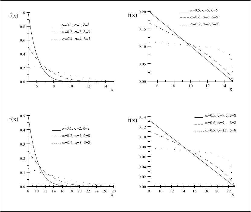
Plots of probability density function for various values of parameters
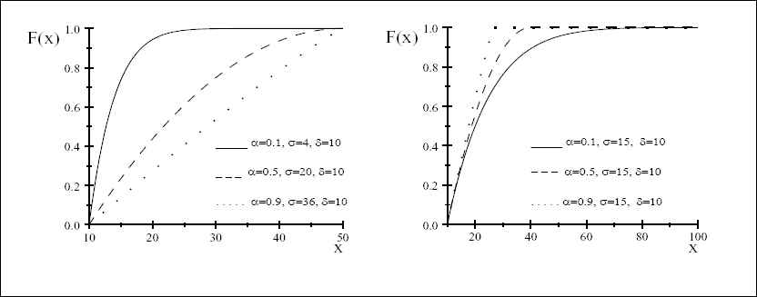
Plots of distribution function for various values of parameters
3. Estimation of the Parameters
3.1 Maximum Likelihood Method
In this section we briefly discuss the maximum likelihood estimators, see Bickel and Docksum [2]. Let x1, x2,...,xn be a random sample of size n from GE2(α,σ,δ); then the likelihood function, L(α,σ,δ), is given by
3.2 Method of Moments
The r-th raw moment of the generalized exponential distribution, Hossain and Ahsanullah [5], is given by
Theorem 3.1.
The parameters obtained by the method of moments for a (α, δ, σ) generalized exponential distribution to have a unique solution, it is sufficient to show that the sample skewness is bounded between 0 and 2, that is,
Proof.
Equating the sample raw moments with the corresponding population raw moments (Hossain and Ahsanullah [5]) we obtain the following three equations in terms of the parameters α, δ, and σ.
Substituting σ and δ from the equations (7) and (8) into the equation (6), we obtain
Now it comes down to solving a non-linear equation in only one unknown parameter α. Let
4. Application
4.1 Data Analysis
In this section we analyze a set of data that arose in tests on the endurance of deep grove ball bearings. They were discussed by Lieblein and Zelen [8], Gupta and Kundu [3], and Gupta and Kundu [4]. The data are the number of revolutions in millions before failure for each of the 23 ball bearings in the life test and they are –
| 17.88 | 28.92 | 33.00 | 41.52 | 42.12 | 45.60 | 48.40 | 51.84 | 51.96 |
| 54.12 | 55.56 | 67.80 | 68.64 | 68.64 | 68.88 | 84.12 | 93.12 | 98.64 |
| 105.12 | 105.84 | 127.92 | 128.04 | 173.40 |
We have fitted four distributions, namely three-parameter Weibull, three-parameter gamma, and three parameter GE1, and three-parameter GE2 to this data set.
4.1.1 ML estimates
From equation (1) we obtain the ML estimate for location parameter
4.1.2 Method of moments estimates
The sufficient condition for the existence of unique solution is given by
The following TABLE 1 appends the ML estimates of parameters, chi-squared statistics, and the Kolmogorov-Smirnov (K-S) statistics of four three-parameter distributions and the moments estimate of parameters for GE2. The TABLE 2 shows the observed and the expected frequencies. All the distributions fit well to this popular data set. The moment estimates of parameters of GE2 performed better than the other three-parameter distributions with ML estimated parameters except for GE1. The GE1 distribution fitted marginally better than GE2 for this data set.
| χ2 | K − S | ||||
|---|---|---|---|---|---|
| Gamma (MLE) | 2.7316 | 0.0441 | 10.2583 | 0.950 | 0.107 |
| Weibull (MLE) | 1.5979 | 0.0156 | 14.8479 | 1.321 | 0.118 |
| GE1 (MLE) | 4.1658 | 0.0314 | 4.7476 | 0.675 | 0.103 |
| GE2(MLE) | 0.4341 | 77.3300 | 17.8800 | 4.289 | 0.112 |
| GE2(Moments) | 0.2957 | 59.9330 | 25.9650 | 1.557 | 0.185 |
Estimates of parameters for similar three-parameter distributions
| Intervals | Observed | Gamma | Weibull | GE1 | GE2(Moments) | GE2(ML) |
|---|---|---|---|---|---|---|
| 0 – 40 | 3 | 4.493 | 4.738 | 4.322 | 4.956 | 6. 053 |
| 40 – 80 | 12 | 10.658 | 10.016 | 10.913 | 9.984 | 8. 382 |
| 80 – 120 | 5 | 5.423 | 5.627 | 5.303 | 5.268 | 5. 331 |
| 120 – 160 | 2 | 1.805 | 1.992 | 1.739 | 2.201 | 2. 655 |
| 160 – 200 | 1 | 0.621 | 0.627 | 0.723 | 0.560 | 0.381 |
Observed and expected frequencies
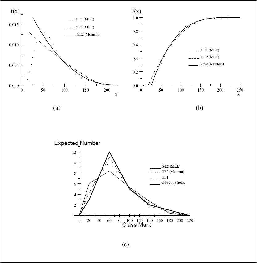
Plots of (a) estimated probability density function, (b) estimated distribution function, and (c) expected values under different models and observed values.
5. Conclusion
This paper offers a new family of three-parameter generalized exponential distribution. The distribution can be used as an alternative to analyzing skewed data. Since the distribution function is in closed form, the inference based on the censored data can be handled by this model more easily than the gamma family distributions.
The model is bounded on both sides by positive values and has an increasing hazard rate function. This makes the model suitable for demographers and actuaries to determine the force of mortality for older age groups.
The Generalized exponential distribution (GE2) is a right skewed unimodal density function. Its hazard function is monotonically increasing for 0 < α < 1. The one real life example used in this article shows that this distribution can quite effectively be used to analyze lifetime data in place of generalized gamma, generalized Weibull and generalized exponential (GE1) distributions. This three-parameter GE2 distribution is always as flexible as the three-parameter GE1, Weibull or gamma distributions.
Acknowledgements
The author would like to thank the referees for their valuable comments and suggestions which contributed to improving the write-up of the manuscript.
References
Cite this article
TY  - JOUR
AU  - Syed Afzal Hossain
PY  - 2018
DA  - 2018/09/30
TI  - Estimating the Parameters of a Generalized Exponential Distribution
JO  - Journal of Statistical Theory and Applications
SP  - 537
EP  - 553
VL  - 17
IS  - 3
SN  - 2214-1766
UR  - https://doi.org/10.2991/jsta.2018.17.3.9
DO  - 10.2991/jsta.2018.17.3.9
ID  - Hossain2018
ER  -