
Classical and Bayesian Inference for the Burr Type XII Distribution Under Generalized Progressive Type I Hybrid Censored Sample
- DOI
- 10.2991/jsta.d.201211.001How to use a DOI?
- Keywords
- Burr Type XII distribution; Confidence intervals; EM algorithm; Generalized progressive hybrid censoring; Markov chain Monte Carlo technique
- Abstract
This paper describes the classical and Bayesian estimation for the parameters of the Burr Type XII distribution based on generalized progressive Type I hybrid censored sample. We first discuss the maximum likelihood estimators of unknown parameters using the expectation-maximization (EM) algorithm and associated interval estimates using Fisher information matrix. We then derive the Bayes estimators with respect to different symmetric and asymmetric loss functions. In this regard, we use Lindley's approximation and importance sampling methods. Highest posterior density (HPD) intervals of unknown parameters are constructed as well. The results of simulation studies and real data analysis are conducted to compare the performance of the proposed point and interval estimators.
- Copyright
- © 2020 The Authors. Published by Atlantis Press B.V.
- Open Access
- This is an open access article distributed under the CC BY-NC 4.0 license (http://creativecommons.org/licenses/by-nc/4.0/).
1. INTRODUCTION
The Burr Type XII (BXII) distribution first appears as part of the Burr system of distributions which was introduced by Burr (Burr [1]). The BXII distribution is becoming increasingly used in the contexts of lifetime data analysis, reliability analysis, quality control, insurance risk and actuarial science in order to reduce the likelihood of failure. In the recent past few years, this distribution has gained some attention among researchers, see for example, Gunasekera [2] and Panahi [3]. The probability density function (PDF) and cumulative distribution function (CDF) of the BXII distribution are given by, respectively,
The hazard rate function is
For
For
For
Moreover, There are many situations including reliability and life-testing experiments where observed data are censored in nature. Type I and Type II censoring schemes are the two most commonly used censoring schemes. The hybrid censoring scheme is a mixture of the Type I and Type II censoring schemes which first introduced by Epstin [4]. Some recent studies on hybrid censoring scheme have been carried out by many authors including Gupta and Singh [5] and Panahi and Sayyareh [6]. One of the traditional defects in the Type I, Type II or hybrid censoring schemes is that they do not allow for removal of units at points other than the final point of the experiment. To deal with this problem, a more general censoring scheme called progressive Type II censoring (PC) has been introduced. Moreover, Kundu and Joarder [7] proposed the progressive hybrid censoring (PHC) scheme. Many authors have discussed the estimation procedure under PC and PHC schemes. See, for example, Lin et al. [8], Panahi [9].
One limitation of the PHC scheme is that it cannot be applied when very few failures may occur before time T. So, Cho et al. [10] introduced generalized progressive hybrid censoring scheme (GPHCS) which not only control the experiment within a proper testing period, but also guarantee certain number of failures in testing procedure. It can be described as follows. Suppose that
Note that for Case 2,
The generalized progressive hybrid censored samples have been investigated for instance by Cho et al. [11], Gorny and Cramer [12], Koley and Kundu [13] and Mohie El-Din et al. [14]. In this paper, we consider the analysis of generalized progressive hybrid censored lifetime data when the lifetime of each experimental unit follows a BXII distribution, and we try to compute the MLE's and Bayesian estimates of the unknown parameters. The rest of the paper is organized as follows: In Section 2, we obtain the maximum likelihood estimators of the unknown parameters of the BXII distribution using the EM algorithm. Using missing information principle, the asymptotic confidence intervals are also constructed. In Section 3, the Bayesian estimates are computed using Lindley's and Markov Chain Monte Carlo (MCMC) techniques. The highest posterior density (HPD) credible intervals with some calculations are also constructed as well. Simulation results of the different methods are presented in Section 4. A real set of data is analyzed in Section 5, and in Section 6, we conclude the paper.
2. EM ALGORITHM
Let
Here,
Here
Here
It is observed that it is difficult to solve likelihood equations analytically due to the associated form of likelihood function. So, we use the EM algorithm (Dempster et al. [15]) to compute them. Suppose that
The E-step of the EM-iteration needs the following conditional expectations:
The M-step in a EM-iteration is maximizing the likelihood function based on complete sample over
Further, we show the existence and uniqueness of the ML estimates of the parameters of the BXII distribution based on GPHCS data using the graphical method (Ateya [16]) as follows:
- ♢
Choose certain Case of censored data as
- ♢
Plot the curves of the equations
- ♢
Figure 1 indicates that there exist one intersection point (1.0029, 1.1202). So, we can say that the solution of the
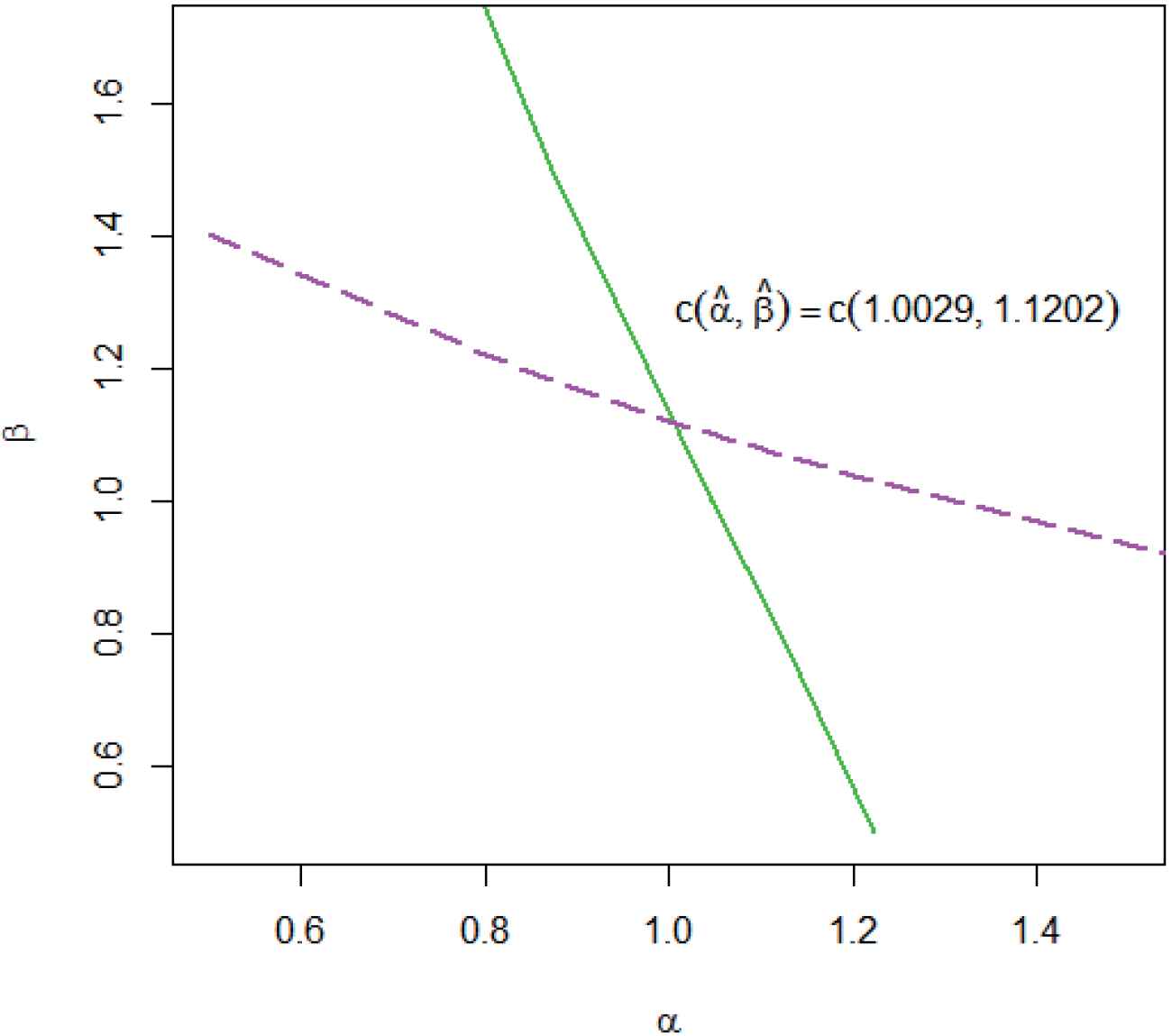
maximum likelihood estimator (MLEs) of
2.1. Approximate Confidence Interval
In this subsection, we obtain the observed Fisher information matrix
Further, we have
Therefore, the expected missing information can then be computed as
3. BAYESIAN ETIMATION
3.1. The Prior and Posterior Distributions
In this section, we discuss Bayesian estimates of the unknown parameters of the BXII distribution under GPHCS using the squared error (SE) and linex (LI) loss functions. These loss functions are defined as, respectively,
Here
Therefore,
Similarly for the LI loss function, we have
Unfortunately, we cannot obtain (10) and (11) analytically. So, we propose two approximation methods for evaluating the Bayes estimates of
3.2. Lindley's Approximation
In this section, Lindley's approximation (Lindley [17]) is applied to gain Bayes estimates of
Also, the Bayesian estimate of
Moreover,
3.3. MCMC Method and HPD Credible Intervals
The MCMC methodology serves as an effective tool for generating random samples on complex Bayesian models. The importance sampling method provides commonly used in MCMC methods. So, we use this method to compute the Bayes estimates and construct the HPD credible intervals of unknown parameters. Based on the independent proposed priors, the posterior density functions of
We propose the following algorithm along the line of Kundu and Pradhan [18] to compute the Bayes estimate of
- Step I:
Generate
- Step II:
Given
- Step III:
Repeat Steps I and II, M times to obtain the importance sample
- Step IV:
The Bayes estimate of
andWe also construct the HPD intervals of
4. SIMULATION STUDY
In this section, we present simulation study to compare the performance of the classical and Bayesian estimation procedures under different GPHCS. Extensive computations were performed using statistical software R. We simulate GPHCS for different combinations of
By employing an EM algorithm, the maximum likelihood estimates have been computed. Approximate expressions for the Bayesian estimators have been computed using the Lindley's approximation and importance sampling algorithm. The Bayes estimates are obtained by assuming that
- Scheme 1:
- Scheme 2:
- Scheme 3:
The average estimates, mean squared errors (MSEs) and average confidence intervals based on 10000 replications have been reported in Tables 1–3. For more compression, the MSEs of the proposed estimators and lengths of intervals are presented in Figures 2 and 3 for some values of generalized progressive censoring schemes.
| Lindely |
MCMC |
||||||
|---|---|---|---|---|---|---|---|
| T = .9 | (24, 12) | 1.7870 (.6999) | 1.6439 (.6644) | 1.4997 (.5844) | 1.5651 (.3525) | 1.4912 (.3414) | |
| n = 30 | 1.8548 (.7231) | 1.7212 (.6538) | 1.5618 (.4471) | 1.7412 (.4444) | 1.6368 (.3961) | ||
| 1.7021 (.5263) | 1.5774 (.3862) | 1.4312 (.3060) | 1.6041 (.3052) | 1.5357 (.2329) | |||
| (28, 12) | 1.5119 (.6467) | 1.3923 (.4457) | 1.2678 (.3655) | 1.4384 (.2432) | 1.3575 (.2370) | ||
| 1.5663 (.5489) | 1.4121 (.4812) | 1.2939 (.3922) | 1.4603 (.3255) | 1.3788 (.2373) | |||
| 1.4927 (.4066) | 1.3777 (.3473) | 1.2556 (.2514) | 1.4246 (.2321) | 1.3451 (.1389) | |||
| T = 1 | (24, 12) | 1.7182 (.5769) | 1.6418 (.4570) | 1.4806 (.3513) | 1.6236 (.3370) | 1.5475 (.2446) | |
| n = 30 | 1.8393 (.6847) | 1.7239 (.4616) | 1.5615 (.3465) | 1.6882 (.3277) | 1.5584 (.2440) | ||
| 1.7029 (.5123) | 1.5905 (.2933) | 1.4414 (.1989) | 1.7067 (.1768) | 1.6324 (.1248) | |||
| (28, 12) | 1.4220 (.4306) | 1.3540 (.3243) | 1.2144 (.2201) | 1.2542 (.1841) | 1.2018 (.1704) | ||
| 1.4568 (.3791) | 1.3747 (.2902) | 1.2320 (.2531) | 1.2941 (.2176) | 1.2418 (.1925) | |||
| 1.3962 (.3855) | 1.3402 (.2150) | 1.2017 (.1682) | 1.2780 (.0751) | 1.2260 (.0602) | |||
| T = .9 | (32, 16) | 1.7247 (.5141) | 1.6220 (.3250) | 1.4906 (.2150) | 1.5993 (.1362) | 1.5580 (.1257) | |
| n = 40 | 1.8944 (.9081) | 1.7145 (.4315) | 1.5908 (.3708) | 1.6325 (.2787) | 1.5780 (.2133) | ||
| 1.6594 (.4087) | 1.5770 (.2637) | 1.4568 (.1863) | 1.5077 (.1503) | 1.4599 (.1230) | |||
| (36,16) | 1.5045 (.3809) | 1.4157 (.2590) | 1.3130 (.2038) | 1.4165 (.0977) | 1.3797 (.0828) | ||
| 1.5684 (.5176) | 1.4512 (.3918) | 1.3496 (.3094) | 1.3804 (.2075) | 1.3391 (.1642) | |||
| 1.4471 (.2380) | 1.3869 (.1339) | 1.2790 (.1103) | 1.3823 (.0712) | 1.3459 (.0582) | |||
| T = 1 | (32, 16) | 1.7346 (.4949) | 1.6435 (.3156) | 1.5095 (.2161) | 1.6531 (.1681) | 1.6097 (.1308) | |
| n = 40 | 1.8297 (.6762) | 1.7060 (.4281) | 1.5606 (.2977) | 1.7220 (.2417) | 1.6638 (.2021) | ||
| 1.6586 (.3726) | 1.5899 (.2311) | 1.4659 (.1769) | 1.5375 (.1456) | 1.4897 (.1215) | |||
| (36, 16) | 1.4447 (.1892) | 1.3963 (.1309) | 1.2798 (.0990) | 1.4240 (.0926) | 1.3856 (.0750) | ||
| 1.7434 (.2320) | 1.4154 (.1499) | 1.2941 (.1057) | 1.4356 (.0947) | 1.3925 (.0752) | |||
| 1.4352 (.1791) | 1.3904 (.1226) | 1.2795 (.0865) | 1.3913 (.0621) | 1.3537 (.0478) | |||
MSE, mean squared error; MCMC, Markov Chain Monte Carlo.
The mean values of MLEs and Bayesian estimates along with associated MSEs.
| Lindely |
MCMC |
||||||
|---|---|---|---|---|---|---|---|
| T = .9 | (24, 12) | 1.6759 (.2715) | 1.5907 (.2510) | 1.4981 (.2375) | 1.4024 (.2239) | 1.2732 (.1902) | |
| n = 30 | 1.0707 (.2578) | 1.6108 (.1995) | 1.5180 (.0925) | 1.3765 (.0869) | 1.3553 (.0710) | ||
| 1.6516 (.1828) | 1.6078 (.1733) | 1.4826 (.1543) | 1.5411 (.1422) | 1.5069 (.1396) | |||
| (28, 12) | 1.6335 (.2568) | 1.5948 (.2397) | 1.4439 (.2090) | 1.3297 (.1964) | 1.3054 (.1701) | ||
| 1.6472 (.1701) | 1.5892 (.1557) | 1.4527 (.0975) | 1.3607 (.0634) | 1.3343 (.0590) | |||
| 1.6274 (.1691) | 1.5961 (.1596) | 1.4416 (.0900) | 1.3271 (.0820) | 1.3022 (.0785) | |||
| T = 1 | (24, 12) | 1.6759 (.1499) | 1.6347 (.1437) | 1.4997 (.1128) | 1.4887 (.1060) | 1.4560 (.1030) | |
| n = 30 | 1.7098 (.1768) | 1.6212 (.1589) | 1.5205 (.0914) | 1.6106 (.0683) | 1.3868 (.0606) | ||
| 1.6565 (.1315) | 1.6272 (.1211) | 1.4879 (.0854) | 1.5331 (.0726) | 1.5059 (.0697) | |||
| (28, 12) | 1.6153 (.1418) | 1.6314 (.1403) | 1.4325 (.1011) | 1.4021 (.0937) | 1.3570 (.0834) | ||
| 1.6227 (.1563) | 1.6302 (.1457) | 1.4356 (.0831) | 1.3666 (.0552) | 1.3383 (.0517) | |||
| 1.6085 (.1259) | 1.6317 (.1176) | 1.4297 (.0708) | 1.4309 (.0648) | 1.3846 (.0530) | |||
| T = .9 | (32, 16) | 1.6361 (.1052) | 1.5989 (.1946) | 1.5019 (.0855) | 1.4099 (.0725) | 1.3994 (.0636) | |
| n = 40 | 1.6684 (.1300) | 1.5743 (.1286) | 1.5233 (.0750) | 1.5387 (.0359) | 1.5216 (.0337) | ||
| 1.6260 (.0945) | 1.6009 (.0873) | 1.4992 (.0796) | 1.4178 (.0694) | 1.4044 (.0611) | |||
| (36, 16) | 1.6022 (.1007) | 1.5775 (.0993) | 1.4227 (.0673) | 1.4507 (.0667) | 1.4338 (.0557) | ||
| 1.6145 (.1124) | 1.5697 (.1051) | 1.4694 (.0718) | 1.5238 (.0278) | 1.5028 (.0258) | |||
| 1.5905 (.0921) | 1.5868 (.0825) | 1.4559 (.0638) | 1.4478 (.0642) | 1.4293 (.0624) | |||
| T = 1 | (32, 16) | 1.6500 (.1037) | 1.6274 (.0965) | 1.5168 (.0618) | 1.4669 (.0614) | 1.4548 (.0508) | |
| n = 40 | 1.6672 (.1186) | 1.6251 (.1044) | 1.5247 (.0684) | 1.5429 (.0510) | 1.5209 (.0419) | ||
| 1.6326 (.0886) | 1.6235 (.0872) | 1.5076 (.0645) | 1.4682 (.0545) | 1.4515 (.0529) | |||
| (36, 16) | 1.6064 (.0917) | 1.5931 (.0874) | 1.4575 (.0596) | 1.4894 (.0434) | 1.4692 (.0334) | ||
| 1.6003 (.0982) | 1.6093 (.0959) | 1.4600 (.0622) | 1.5184 (.0244) | 1.4916 (.0214) | |||
| 1.5942 (.0852) | 1.6074 (.0787) | 1.4625 (.0616) | 1.4916 (.0488) | 1.4678 (.0425) | |||
MSE, mean squared error; MCMC, Markov Chain Monte Carlo.
The mean values of MLEs and Bayesian estimates along with associated MSEs.
| ACI | ACI | ||||||
|---|---|---|---|---|---|---|---|
| T = .9 | (24, 12) | (.9344, 2.7197) | (.8375, 2.3375) | (.9800, 2.2939) | (.4902, 1.4964) | ||
| n = 30 | (.9654, 2.9061) | (.9122, 2.2947) | (1.0448, 2.3448) | (.4103, 1.3928) | |||
| (.9091, 2.4950) | (.7390, 1.8992) | (.8581, 2.2480) | (.5074, 1.5712) | ||||
| (28, 12) | (.7567, 2.2823) | (.5909, 1.9019) | (.9972, 2.2699) | (.6274, 1.3527) | |||
| (.7650, 2.3676) | (.7010, 1.9810) | (1.0017, 2.2927) | (.4704, 1.4206) | ||||
| (.7562, 2.2291) | (.8193, 1.8892) | (.9983, 2.2566) | (.4084, 1.3584) | ||||
| T = 1 | (24, 12) | (.9397, 2.6172) | (.9236, 2.005) | (.9914, 2.2393) | (.7703, 1.5099) | ||
| n = 30 | (.9701, 2.8885) | (.9108, 2.1780) | (1.0738, 2.3458) | (.6580, 1.5680) | |||
| (.9279, 2.4779) | (1.0181, 2.0732) | (.9868, 2.2468) | (.6903, 1.5560) | ||||
| (28, 12) | (.7395, 2.1049) | (.7718, 1.6812) | (.9914, 2.2393) | (.6553, 1.4315) | |||
| (.7436, 2.1699) | (.5731, 1.7665) | (.9906, 2.2547) | (.6577, 1.4760) | ||||
| (.7385, 2.0540) | (.8062, 1.7203) | (.9924, 2.2247) | (.6855, 1.4748) | ||||
| T = .9 | (32, 16) | (1.0002, 2.4490) | (.8962, 1.8438) | (1.1108, 2.3608) | (.7789, 1.6099) | ||
| n = 40 | (.9412, 2.7433) | (.1307, 1.2828) | (1.1205, 2.2163) | (.6769, 1.5792) | |||
| (.9926, 2.3262) | (.8434, 1.8434) | (.8856, 2.1356) | (.6478, 1.4578) | ||||
| (36, 16) | (.8564, 2.1526) | (.8331, 1.7041) | (1.0656, 2.1389) | (.8282, 1.4961) | |||
| (.8697, 2.2672) | (.7225, 1.7225) | (1.1205, 2.2163) | (.6769, 1.5792) | ||||
| (.8438, 2.0504) | (.8360, 1.8347) | (.8856, 2.1356) | (.6478, 1.4578) | ||||
| T = 1 | (32, 16) | (1.0272, 2.4420) | (.9564, 1.7657) | (1.1267, 2.1733) | (.8402, 1.4860) | ||
| n = 40 | (1.0441, 2.6153) | (.9800, 2.1277) | (1.1241, 2.2104) | (.7897, 1.5510) | |||
| (1.0113, 2.3059) | (1.0161, 1.8946) | (1.1267, 2.1385) | (.9484, 1.6682) | ||||
| (36, 16) | (.8475, 2.0420) | (.7461, 1.4314) | (1.0645, 2.1216) | (.8135, 1.4988) | |||
| (.8484, 2.0984) | (.8712, 1.8350) | (1.0617, 2.1388) | (.7665, 1.5244) | ||||
| (.8546, 2.0141) | (.8851, 1.7370) | (1.1143, 2.1146) | (.8303, 1.5211) | ||||
ACI, approximate confidence interval; HPD, highest posterior density.
The ACIs and HPD credible intervals for
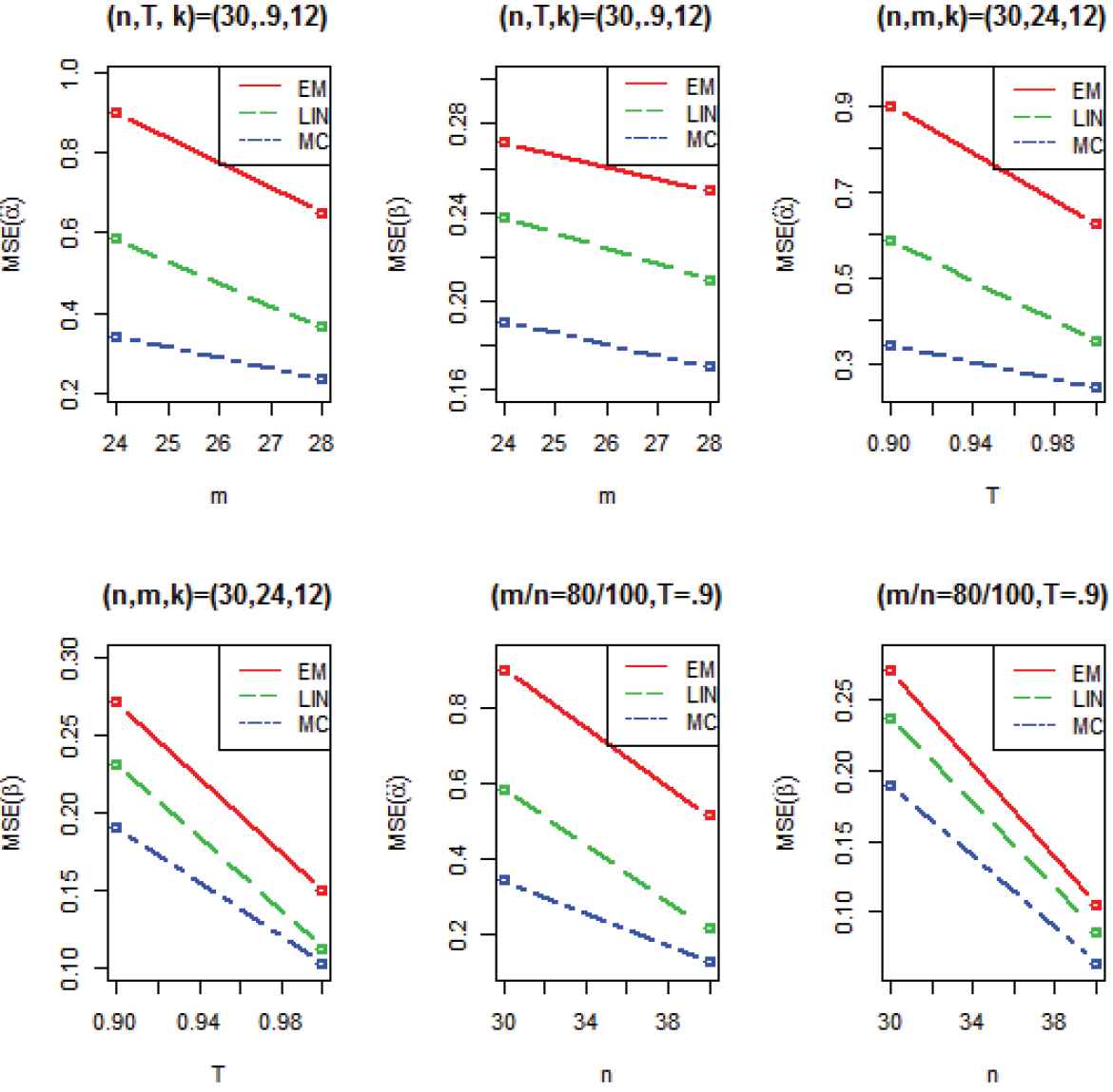
The mean squared errors (MSEs) of the proposed estimators (expectation-maximization (EM), Lindley, Markov Chain Monte Carlo (MCMC)) for different choices of n, T and m.
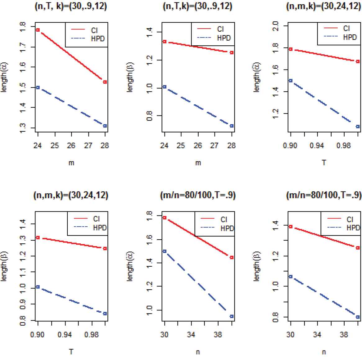
The length of approximate confidence intervals (ACIs) and highest posterior densities (HPDs) for different choices of n, T and m.
It can be observed that for fixed
For fixed
Tabulated values also show that the importance sampling estimates are better choice among all rivals and for all values of
Thus, we recommend Bayesian point and interval estimations of the parameters using importance sampling algorithm.
5. REAL DATA ANALYSIS
In order to illustrate all the inferential results established for the BXII distribution, we analyze one data set from Wingo [20]. We first make an inference whether the BXII distribution fits the given data set. For this purpose, we compute the Kolmogorov-Smirnov (K-S) distances between the empirical distribution and the fitted distribution functions based on MLEs, it is
- Case 1:
- Case 2:
- Case 3:
The maximum likelihood estimates and the approximate Bayesian estimates using Lindley's approximation and MCMC algorithm are presented in Table 4. The upper and lower bounds for the
| Lindely |
MCMC |
||||||
|---|---|---|---|---|---|---|---|
| Case 1: |
16 | .8 | 4.48017 | 4.3678 | 3.6591 | 3.8213 | 3.4523 |
| Case 2: |
8 | 1 | 2.8606 | 2.8167 | 2.3670 | 2.6084 | 2.4212 |
| Case 3: |
8 | 2 | 2.9191 | 2.8879 | 2.5179 | 2.8658 | 2.6769 |
| Case 1: |
16 | .8 | 6.8144 | 7.3354 | 6.0906 | 5.4495 | 5.2748 |
| Case 2: |
8 | 1 | 5.8888 | 6.2755 | 5.2147 | 4.9963 | 4.7647 |
| Case 3: |
8 | 2 | 5.9872 | 6.1919 | 5.4047 | 5.7884 | 5.3493 |
MCMC, Markov Chain Monte Carlo.
The MLEs and Bayesian estimates of
| %95 ACIs | HPD Credible Intervals | ||||
|---|---|---|---|---|---|
| Case 1: |
16 | .8 | (1.9531, 7.0070) | (1.4170, 4.3683) | |
| Case 2: |
8 | 1 | (1.2622, 5.8302) | (1.0755, 3.1945) | |
| Case 3: |
8 | 2 | (1.5281, 4.3101) | (1.4502, 3.8189) |
ACI, approximate confidence interval; HPD, highest posterior density.
The ACIs and HPD intervals of
| %95 ACIs | HPD Credible Intervals | ||||
|---|---|---|---|---|---|
| Case 1: |
16 | .8 | (4.4475, 9.1813) | (3.3368, 6.2481) | |
| Case 2: |
8 | 1 | (3.6823, 8.0954) | (3.8160, 5.9253) | |
| Case 3: |
8 | 2 | (3.8680, 6.8192) | (3.7736, 6.0916) |
ACI, approximate confidence interval; HPD, highest posterior density.
The ACIs and HPD intervals of
6. CONCLUSIONS
In this paper, different point and interval estimation problems have taken into consideration under classical and Bayesian framework when lifetime data following BXII distribution are observed under GPHCS. It is observed that the MLEs cannot be derived in the closed form and instead the traditional Newton-Raphson algorithm, we suggest the EM algorithm to compute them. By applying two different approximation approaches like Lindley's and the importance sampling algorithm, the Bayesian estimates of the parameters under different symmetric and asymmetric loss functions have been obtained. Based on the EM framework and MCMC technique, the confidence intervals have also been constructed. We compared performance of different proposed estimators using Monte Carlo simulations and observed that the Bayes estimates based on importance sampling algorithm outperforms other proposed estimators. An illustrative example is also provided in support of the proposed methods.
ACKNOWLEDGMENTS
The authors are grateful to the Editor in chief and an anonymous referee for making many helpful comments and suggestions on an earlier version of this paper. We also would like to express my deepest appreciation to Professor Gholamhossein Hamedani.
REFERENCES
Cite this article
TY  - JOUR
AU  - Parya Parviz
AU  - Hanieh Panahi
PY  - 2020
DA  - 2020/12/18
TI  - Classical and Bayesian Inference for the Burr Type XII Distribution Under Generalized Progressive Type I Hybrid Censored Sample
JO  - Journal of Statistical Theory and Applications
SP  - 547
EP  - 557
VL  - 19
IS  - 4
SN  - 2214-1766
UR  - https://doi.org/10.2991/jsta.d.201211.001
DO  - 10.2991/jsta.d.201211.001
ID  - Parviz2020
ER  -