
Marshall–Olkin Power Generalized Weibull Distribution with Applications in Engineering and Medicine
- DOI
- 10.2991/jsta.d.200507.004How to use a DOI?
- Keywords
- Marshall–Olkin-G Family; Maximum likelihood; Momemts; Power-generalized Weibull model
- Abstract
This paper proposes a new flexible four-parameter model called Marshall–Olkin power generalized Weibull (MOPGW) distribution which provides symmetrical, reversed-J shaped, left-skewed and right-skewed densities, and bathtub, unimodal, increasing, constant, decreasing, J shaped, and reversed-J shaped hazard rates. Some of the MOPGW structural properties are discussed. The maximum likelihood is utilized to estimate the MOPGW unknown parameters. Simulation results are provided to assess the performance of the maximum likelihood method. Finally, we illustrate the importance of the MOPGW model, compared with some rival models, via two real data applications from the engineering and medicine fields.
- Copyright
- © 2020 The Authors. Published by Atlantis Press SARL.
- Open Access
- This is an open access article distributed under the CC BY-NC 4.0 license (http://creativecommons.org/licenses/by-nc/4.0/).
1. INTRODUCTION
The Weibull distribution has been used in modeling lifetime data with monotonic failure rates. It does not provide adequate fits to real data with unimodal or bathtub-shaped hazard rates, often encountered in engineering, medicine and reliability fields. Hence, several authors have constructed different generalizations and extended forms of the Weibull distribution to increase its flexibilty. For example, exponentiated Weibull [1], Marshall–Olkin extended Weibull [2], beta Weibull [3], Kumaraswamy Weibull [4], transmuted complementary Weibull geometric [5], Weibull-Weibull [6], odd log-logistic exponentiated Weibull [7], alpha logarithmic transformed Weibull [8], and odd Lomax Weibull [9] distributions.
Another Weibull extension called the power generalized Weibull (PGW) model pioneered by [10] and they used it in accelerated failure time models. The hazard rate function (HRF) of PGW model can be monotone, unimodal, and bathtub shaped.
The PGW model can be specified by the cumulative distribution function (CDF)
The corresponding probability density function (PDF) and HRF take the forms,
Some special cases of the PGW distribution are the Weibull distribution with parameters
This paper is devoted to propose and study a new flexible extension of the PGW model called the MOPGW distribution, which has some desirable motivations as follows:
The MOPGW contains a number of well-known lifetime sub-models called, Marshall–Olkin Weibull [15], Marshall–Olkin-NH [16], NH [11], PGW [10], Weibull [17], exponential, and Rayleigh distributions, among others, see Table 1.
The PDF of the MOPGW distribution can be reversed-J shaped, right-skewed, concave down, left-skewed, or symmetric, see Figure 1. Further, its HRF takes some important forms such as, constant, monotone (decreasing or increasing), bathtub, upside down bathtub, and reversed-J shaped. Hence, the MOPGW distribution can be considered as a superior lifetime distribution to other models, which exhibit only monotonic and constant hazard rates, see Figure 2.
The MOPGW distribution is considered as a suitable model for modeling skewed data that cannot be properly modeled by other extensions of the Weibull distribution. Further, it can be utilized to model real data in many applied areas, such as engineering, survival analysis, medicine, and industrial reliability.
The kurtosis of the MOPGW distribution is more flexible as compared to the baseline PGW model, whereas its skewness varies within the interval (1.43529, 5.62470), whereas the PGW skewness can only range in the interval (-0.68927, 4.25756). Further, the MOPGW distribution can be leptokurtic (kurtosis
Two real-life data applications from the engineering and medicine sciences, prove that the MOPGW distribution outperforms nine other well-known competing lifetime distributions, motivating its usage in applied fields.
| Distribution | Authors | ||||
|---|---|---|---|---|---|
| – | – | 1 | – | MO-Weibull | [15] |
| – | 1 | 1 | – | MO-Exponential | [15] |
| – | 2 | 1 | – | MO-Rayleigh | – |
| – | 1 | – | – | MO-NH | [16] |
| – | – | – | 1 | PGW | [10] |
| – | – | 1 | 1 | Weibull | [17] |
| – | 1 | 1 | 1 | Exponential | – |
| – | 2 | 1 | 1 | Rayleigh | [21] |
| – | 1 | – | 1 | NH | [11] |
MOPGW, Marshall-Olkin power generalized Weibull; MO, Marshall-Olkin; NH, Nadarajah-Haghighi; PGW, power generalized Weibull.
Special cases of the MOPGW distribution.
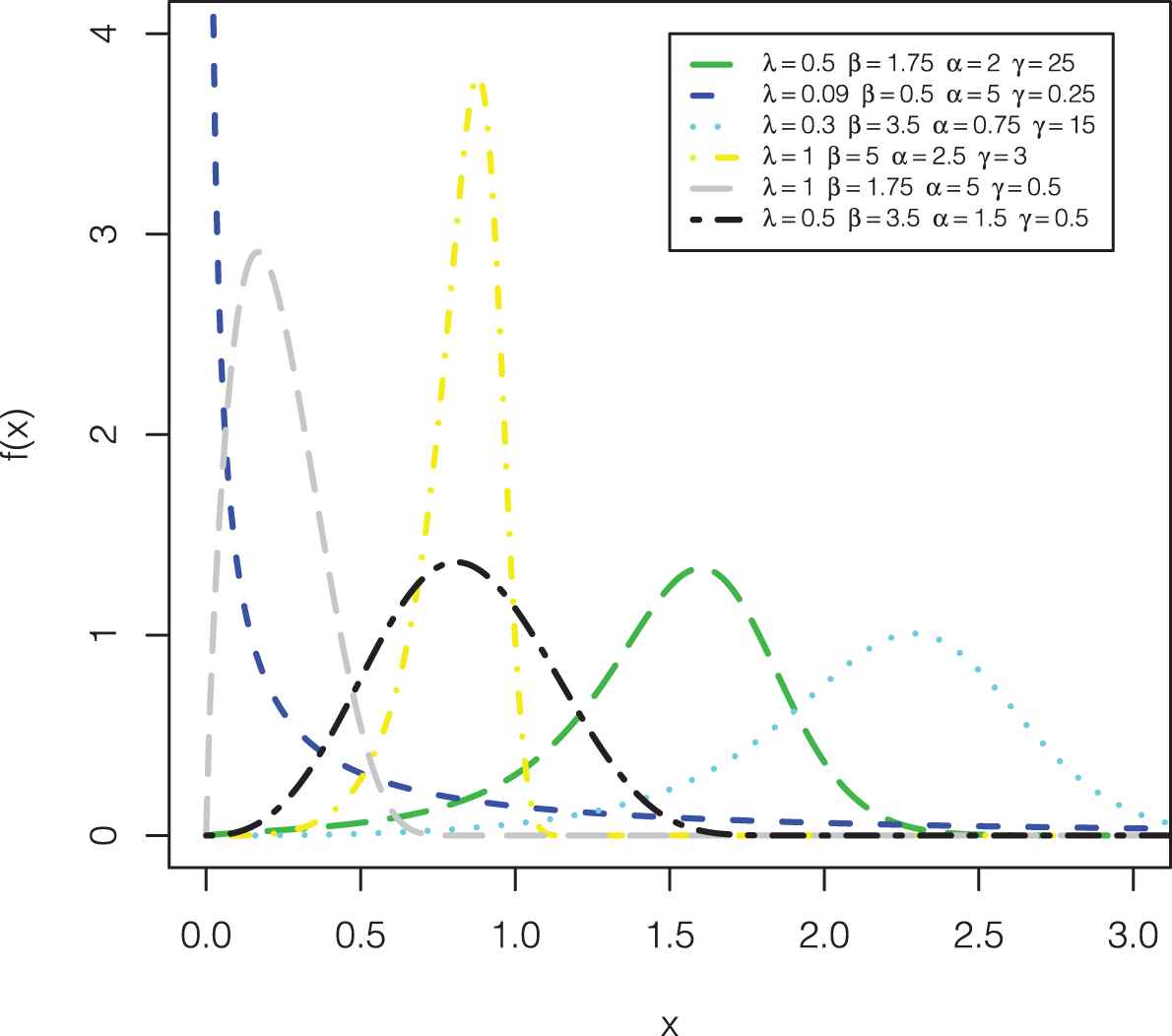
Probability density function (PDF) shapes for the Marshall–Olkin power generalized Weibull (MOPGW) distribution considering different values of its parameters.
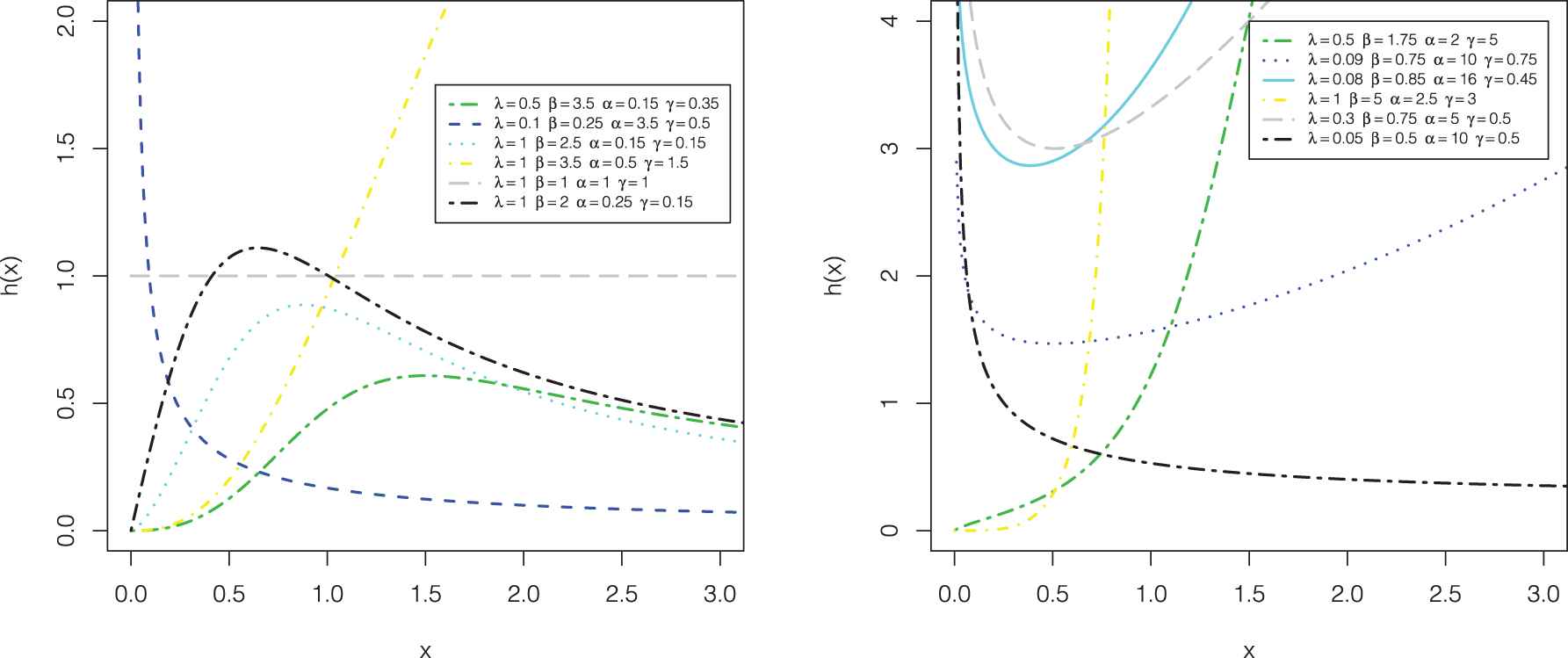
Hazard rate function (HRF) shapes for the Marshall–Olkin power generalized Weibull (MOPGW) distribution considering different values of its parameters.
| 0.5 | 0.5 | 0.5 | 2.83608 | 30.1952 | 2.69914 | 10.2286 |
| 1.5 | 4.22743 | 47.3561 | 1.92163 | 5.88874 | ||
| 5.0 | 3.77437 | 51.0655 | 2.02701 | 6.09045 | ||
| 1.5 | 0.5 | 0.32446 | 0.53667 | 5.62470 | 55.9161 | |
| 5.0 | 1.45888 | 2.59897 | 2.40956 | 13.0233 | ||
| 5.0 | 0.5 | 0.01676 | 0.00084 | 3.39967 | 20.1131 | |
| 5.0 | 0.06375 | 0.00291 | 1.27168 | 5.17103 | ||
| 1.5 | 0.5 | 0.5 | 1.51528 | 2.77558 | 3.00036 | 18.1059 |
| 1.5 | 2.54943 | 5.08931 | 2.11351 | 10.5501 | ||
| 5.0 | 4.16067 | 8.48966 | 1.46293 | 6.80443 | ||
| 1.5 | 0.5 | 0.47876 | 0.11798 | 1.11729 | 4.28686 | |
| 1.5 | 0.70459 | 0.15479 | 0.55711 | 3.02953 | ||
| 5.0 | 0.98220 | 0.17173 | 0.07453 | 2.76358 | ||
| 5.0 | 0.5 | 0.19101 | 0.01481 | 0.72482 | 3.05190 | |
| 1.5 | 0.27045 | 0.01725 | 0.16615 | 2.44296 | ||
| 5.0 | 0.36019 | 0.01646 | −0.35840 | 2.76453 | ||
| 5.0 | 0.5 | 0.5 | 1.02414 | 0.09972 | 0.50451 | 3.35065 |
| 1.5 | 1.22535 | 0.11075 | 0.16575 | 2.98447 | ||
| 5.0 | 1.45201 | 0.10985 | −0.17619 | 3.10095 | ||
| 1.5 | 0.5 | 0.75476 | 0.03309 | −0.17730 | 2.74402 | |
| 1.5 | 0.86456 | 0.02914 | −0.59094 | 3.26362 | ||
| 5.0 | 0.97071 | 0.02195 | −1.04886 | 4.61832 | ||
| 5.0 | 0.5 | 0.57806 | 0.01664 | −0.39356 | 2.82240 | |
| 1.5 | 0.65379 | 0.01351 | −0.86979 | 3.74856 | ||
| 5.0 | 0.72281 | 0.00917 | −1.43529 | 5.93460 |
MOPGW, Marshall-Olkin power generalized Weibull.
μ, σ2, γ1, and γ2 of the MOPGW model for several values of its parameters with λ = 1.
The MOPGW distribution is constructed by incorporating the PGW as a baseline model in the Marshall–Olkin-G (MO-G) family proposed by [15]. This family has been widely used to provide more flexible extensions of the well-known classical distributions in the statistical literature. See, for example, [2,18,19], and the references therein.
The CDF of the MO-G family has the form
The corresponding PDF and HRF of the MO-G class are
The rest of the article is outlined as follows: The MOPGW distribution, its special cases, and PDF and HRF plots are provided in Section 2. Several structural properties of the MOPGW distribution are derived in Section 3. In Section 4, the estimation of the MOPGW parameters is demonstrated via the maximum likelihood and its performance is evaluated by simulation results. In Section 5, we illustrate the importance of the MOPGW model by using two real data applications. Finally, the paper is concluded in Section 6.
2. THE MOPGW DISTRIBUTION
In this section, we introduce the four-parameter MOPGW distribution. By inserting (1) in Equation (2), the CDF of the MOGPW distribution follows as
The corresponding PDF of the MOPGW distribution takes the form
Henceforth, the random variable with PDF (4) is denoted by
The HRF of the MOPGW distribution reduces to
Figures 1 and 2 display some plots of the probability density and hazard functions of the MOPGW distribution for some different values of its parameters. Figures 1 and 2 reveal that the MOGPW density exhibits reversed-J shaped, left-skewed, symmetric, or right-skewed shapes, whereas its HRF can exhibit constant, monotone (increasing or decreasing), or nonmonotone (unimodal or bathtub) hazard rate shapes.
Further, the MOPGW distribution contains some important special sub-models which are displayed in Table 1.
3. STATISTICAL PROPERTIES OF THE MOPGW DISTRIBUTION
Some properties of the MOPGW distribution including quantile function (QF), ordinary and conditional moments, generating function (MGF), mean deviation, Lorenz and Bonferroni curves, and residual life and reversed residual life moments are derived.
3.1. Quantile Function
The QF
Equation (5) can be easily used to generate the MOPGW random variates, and the median of
3.2. Moments
Here, we derive the
Theorem 1.
If
Proof:
The
Using the generalized binomial expression for
Using Equation (7) in (6), we obtain
Setting
Consider the power series with real number power
Table 2 shows some numerical values for the mean,
3.3. Generating Function
The MGF is useful for several reasons, one of which is its application in analyzing the sums of random variables.
Theorem 2.
If
Proof.
The MGF can be defined as
Since the series expansion of
Then, substituting from Equations (10) into (11), we get
3.4. Conditional Moments
The
After some algebra, we get
Similarly, the
The
3.5. Mean Deviation, Lorenz, and Bonferroni Curves
This section is devoted to derive the mean deviation about the mean, denoted by
The mean deviations about the mean of the MOPGW distribution is
The mean deviations about the median of the MOPGW distribution has the form
Using Equation (10), we get the mean of
Further, the Lorenz and Bonferroni curves have useful applications in income inequality measures, demography, reliability, insurance, and medicine.
Lorenz curve has the form
The Bonferroni curve takes the form
3.6. Moments of Residual and Reversed Residual Lives
The
Using the binomial series to the term
The mean residual life (MRL) of the MOPGW distribution follows from the last equation, with
The variance residual life of the MOPGW distribution is obtained directly using
Further, the
Using the binomial series to the term
The mean waiting time (or mean reversed residual life) of the MOPGW distribution reduces to
The variance and coefficient of variation of reversed residual life for the MOPGW distribution follow simply using
4. ESTIMATION AND SIMULATION
In this section, we discuss the estimation of the MOPGW parameters using the maximum likelihood. Let
The log likelihood function,
The maximum likelihood estimates (MLEs) of
Further, there are some programs called, Ox program (sub-routine MaxBFGS), SAS (PROCNLMIXED), R (optim function), Mathcad, and Newton–Rapshon method, which can be utilized to maximize the log-likelihood function in order to determine the MLEs.
Now, we perform a Monte Carlo simulation to evaluate the performance of the MLEs of the MOPGW parameters
| Parameters |
AVEs |
MSEs |
|||||||||
|---|---|---|---|---|---|---|---|---|---|---|---|
| 0.5 | 0.1 | 0.5 | 1 | 0.9202 | 0.0500 | 0.8640 | 0.9930 | 1.6582 | 0.9753 | 0.0500 | 2.3723 |
| 1 | 1.2811 | 0.0580 | 1.0871 | 2.9701 | 1.1396 | 1.3785 | 0.0541 | 1.4844 | |||
| 1.5 | 1.9702 | 0.1011 | 0.8217 | 2.4601 | 0.4943 | 1.3842 | 0.4189 | 1.1360 | |||
| 2 | 1.3065 | 0.1214 | 0.9389 | 2.7378 | 1.4620 | 1.7830 | 0.1344 | 1.7093 | |||
| 0.3 | 0.5 | 2.2057 | 0.1235 | 0.6703 | 2.7709 | 1.0459 | 1.9742 | 0.0815 | 1.9016 | ||
| 1 | 0.9405 | 0.2207 | 1.0513 | 1.8933 | 0.7882 | 1.4132 | 0.3502 | 2.1485 | |||
| 1.5 | 1.2020 | 0.2977 | 1.2730 | 2.5025 | 0.7177 | 1.4006 | 0.3133 | 1.6867 | |||
| 2 | 1.1791 | 0.3759 | 1.0358 | 2.6856 | 0.5435 | 1.1479 | 0.4736 | 1.3190 | |||
| 1 | 0.1 | 0.5 | 1.5039 | 0.0500 | 0.9729 | 2.7398 | 1.1576 | 0.7366 | 0.2676 | 1.4537 | |
| 1 | 1.9530 | 0.7891 | 0.7961 | 1.7431 | 1.4313 | 0.1478 | 0.9689 | 1.5849 | |||
| 1.5 | 2.0288 | 0.3393 | 1.2637 | 2.9830 | 1.0931 | 0.0707 | 2.0806 | 1.5534 | |||
| 2 | 2.5381 | 1.1032 | 0.9184 | 2.9873 | 1.4982 | 0.0679 | 1.5117 | 2.3054 | |||
| 0.3 | 0.5 | 1.9103 | 0.2057 | 0.6087 | 1.8260 | 1.5463 | 0.7388 | 0.9302 | 1.1497 | ||
| 1 | 2.2046 | 0.5422 | 0.7175 | 2.9335 | 1.9484 | 0.5651 | 0.6425 | 1.8055 | |||
| 1.5 | 3.0120 | 1.3879 | 0.5676 | 3.1894 | 1.5879 | 0.4016 | 1.1681 | 2.2586 | |||
| 2 | 2.1232 | 2.5133 | 1.7885 | 2.9748 | 0.9844 | 0.3422 | 1.8977 | 0.9037 | |||
| 0.5 | 0.1 | 0.5 | 2 | 0.3270 | 0.0500 | 0.6942 | 0.8281 | 0.9630 | 0.4918 | 0.6203 | 1.7827 |
| 1 | 1.1391 | 0.0533 | 1.1584 | 2.7994 | 0.1380 | 1.0959 | 0.5341 | 2.5354 | |||
| 1.5 | 0.9781 | 0.0737 | 1.1984 | 2.9578 | 0.1363 | 2.1470 | 0.0547 | 2.2515 | |||
| 2 | 1.7858 | 0.1049 | 0.7978 | 2.9440 | 0.2439 | 1.9954 | 0.1420 | 2.9927 | |||
| 0.3 | 0.5 | 2.2858 | 0.1029 | 0.6213 | 2.6937 | 0.4588 | 1.4278 | 0.1588 | 2.0491 | ||
| 1 | 2.1103 | 0.1975 | 0.5946 | 2.3362 | 0.3802 | 1.2081 | 0.4836 | 2.1916 | |||
| 1.5 | 2.2977 | 0.2504 | 0.6448 | 2.9056 | 0.3301 | 1.5568 | 0.3173 | 1.7513 | |||
| 2 | 1.5577 | 0.3140 | 1.0508 | 2.8405 | 0.4583 | 1.5468 | 0.4170 | 1.3579 | |||
| 1 | 0.1 | 0.5 | 0.9596 | 0.0510 | 1.0642 | 1.7048 | 1.0923 | 0.6854 | 0.1785 | 1.4263 | |
| 1 | 1.0611 | 0.1292 | 0.9846 | 1.5859 | 1.3129 | 0.2748 | 0.8653 | 0.7359 | |||
| 1.5 | 1.6313 | 0.3118 | 1.1332 | 2.6599 | 1.5714 | 0.1743 | 1.1237 | 1.5683 | |||
| 2 | 2.5047 | 0.8806 | 1.0001 | 2.9519 | 1.3696 | 0.0676 | 1.5708 | 1.4902 | |||
| 0.3 | 0.5 | 0.9017 | 0.1320 | 1.0972 | 1.9979 | 1.1166 | 0.9673 | 0.7618 | 1.7971 | ||
| 1 | 1.2100 | 0.4056 | 0.7544 | 1.6171 | 1.4462 | 0.4686 | 0.6188 | 1.4686 | |||
| 1.5 | 0.8302 | 0.5522 | 1.7014 | 2.8225 | 1.5482 | 0.6256 | 0.8528 | 1.7732 | |||
| 2 | 2.0142 | 1.6809 | 1.5975 | 2.9999 | 1.3241 | 0.4989 | 1.3067 | 1.7950 | |||
AVE, average estimate; MSE, mean squares error.
AVEs and their associated MSEs
| Parameters |
AVEs |
MSEs |
|||||||||
|---|---|---|---|---|---|---|---|---|---|---|---|
| 0.5 | 0.1 | 0.5 | 1 | 0.3595 | 0.0500 | 0.6929 | 0.4942 | 1.0292 | 0.7498 | 0.2392 | 2.1435 |
| 1 | 0.9676 | 0.0580 | 1.2379 | 2.7996 | 1.0687 | 0.9651 | 0.3836 | 1.4553 | |||
| 1.5 | 1.3876 | 0.0985 | 0.9082 | 2.2925 | 0.9067 | 1.8129 | 0.1981 | 1.3743 | |||
| 2 | 1.3068 | 0.1283 | 0.9110 | 2.0583 | 1.0018 | 2.0171 | 0.2020 | 1.2384 | |||
| 0.3 | 0.5 | 1.5576 | 0.2141 | 0.9024 | 2.4123 | 0.7984 | 2.0533 | 0.2072 | 1.8196 | ||
| 1 | 1.6017 | 0.2043 | 0.9302 | 2.5424 | 0.6430 | 1.5325 | 0.3686 | 1.1215 | |||
| 1.5 | 1.4011 | 0.2943 | 1.0464 | 2.3157 | 0.8278 | 1.4305 | 0.3485 | 1.6112 | |||
| 2 | 1.6386 | 0.3782 | 0.9007 | 2.4975 | 0.7073 | 1.9542 | 0.3109 | 1.2240 | |||
| 1 | 0.1 | 0.5 | 1.0035 | 0.0519 | 1.0910 | 2.4792 | 1.2406 | 0.8302 | 0.2642 | 1.1904 | |
| 1 | 2.3296 | 0.5527 | 0.6585 | 2.0968 | 1.8703 | 0.2951 | 0.4097 | 0.7702 | |||
| 1.5 | 2.7437 | 0.4934 | 0.6510 | 2.9925 | 1.3197 | 0.0946 | 1.7443 | 1.5855 | |||
| 2 | 2.0756 | 0.9331 | 1.4044 | 2.9889 | 1.3320 | 0.0658 | 2.0452 | 1.4687 | |||
| 0.3 | 0.5 | 1.6041 | 0.2006 | 0.6433 | 1.5800 | 2.3048 | 1.3419 | 0.2079 | 0.8049 | ||
| 1 | 1.7475 | 0.4622 | 1.0189 | 2.5818 | 1.6972 | 0.4632 | 0.8230 | 1.5771 | |||
| 1.5 | 2.1441 | 0.9269 | 1.1965 | 2.9988 | 1.3120 | 0.4003 | 1.3964 | 1.8371 | |||
| 2 | 1.9626 | 1.7117 | 1.7679 | 2.9993 | 1.2800 | 0.3688 | 1.9772 | 1.6761 | |||
| 0.5 | 0.1 | 0.5 | 2 | 0.2979 | 0.0500 | 0.7382 | 0.8526 | 0.9125 | 0.5190 | 0.3053 | 2.1986 |
| 1 | 1.0792 | 0.0508 | 1.1367 | 2.9312 | 0.4648 | 1.2058 | 0.3080 | 2.4279 | |||
| 1.5 | 1.1903 | 0.0761 | 1.0201 | 2.5770 | 0.5441 | 1.4865 | 0.3016 | 2.2644 | |||
| 2 | 1.5855 | 0.1078 | 0.8191 | 2.1929 | 0.7954 | 2.2353 | 0.1865 | 2.1491 | |||
| 0.3 | 0.5 | 1.3581 | 0.0998 | 0.9561 | 2.2802 | 0.5436 | 2.0943 | 0.1089 | 2.3885 | ||
| 1 | 1.2990 | 0.1881 | 0.9117 | 2.1297 | 0.3253 | 1.8123 | 0.2371 | 2.0485 | |||
| 1.5 | 1.1645 | 0.2507 | 1.1015 | 2.4764 | 0.4894 | 1.9389 | 0.2591 | 2.2461 | |||
| 2 | 1.4522 | 0.3199 | 0.9606 | 2.6714 | 0.5056 | 1.6968 | 0.3897 | 1.8849 | |||
| 1 | 0.1 | 0.5 | 1.5041 | 0.0501 | 0.9779 | 1.6841 | 0.9834 | 0.7566 | 0.3622 | 1.7222 | |
| 1 | 2.2392 | 0.1842 | 0.4764 | 1.3209 | 1.9527 | 0.6950 | 0.3336 | 0.5380 | |||
| 1.5 | 2.2205 | 0.3257 | 0.8010 | 2.7536 | 1.8079 | 0.2037 | 0.9809 | 1.8040 | |||
| 2 | 2.3423 | 0.7380 | 1.0303 | 2.9997 | 1.4461 | 0.0953 | 1.6802 | 1.7298 | |||
| 0.3 | 0.5 | 1.5499 | 0.1429 | 0.8390 | 2.1318 | 1.4969 | 1.5425 | 0.3213 | 1.4146 | ||
| 1 | 1.9087 | 0.4567 | 0.6987 | 1.6015 | 1.9548 | 0.9360 | 0.3987 | 1.1856 | |||
| 1.5 | 2.1028 | 0.8042 | 0.9827 | 2.9339 | 1.3663 | 0.5518 | 1.0519 | 1.6054 | |||
| 2 | 1.9990 | 1.4741 | 1.5191 | 2.9987 | 1.1484 | 0.5384 | 1.7617 | 1.6857 | |||
AVE, average estimate; MSE, mean squares error.
AVEs and their associated MSEs
The values of AVEs and MSEs reveal that
All parameters estimates show consistency property, that is, the MSEs decrease when the sample size increases.
For fixed
For fixed
For fixed
For fixed
5. APPLICATIONS
Two real data applications are provided in this section to study empirically the importance and flexibility of the MOPGW distribution. The first set of data represents the gauge lengths of 20 mm and it consists of
For the gauge lengths and cancer data, the fits of the MOPGW model is compared with some competitive distributions called, the exponentiated power generalized Weibull (EPGW) [32], alpha power exponentiated W (APEW) [33], Kumaraswamy W (KwW) [4], beta W (BW) [3], transmuted geometric W (TGcW [34], transmuted exponentiated generalized W (TEGW) [35], odd Lomax W (OLxW) [9], W Burr XII (WBXII) [36], and W Fréchet(WFr) [37].
The
Tables 5 and 6 provide the MLEs and associated standard errors (SEs) (between parentheses) of the parameters of all fitted models and the values of
| Distribution | Estimates (SEs) | |||||||
|---|---|---|---|---|---|---|---|---|
| MOPGW ( |
0.0287 | 7.1320 | 0.3624 | 6.3451 | 0.0244 | 0.1839 | 0.0503 | 0.9921 |
| (0.0895) | (6.2545) | (0.6108) | (21.620) | |||||
| EPGW ( |
0.0320 | 3.5114 | 1.4106 | 2.1014 | 0.0269 | 0.2119 | 0.0580 | 0.9648 |
| (0.0661) | (4.4837) | (3.1836) | (2.7709) | |||||
| APEW ( |
5.5281 | 3.3500 | 0.0863 | 2.1428 | 0.0256 | 0.1911 | 0.0521 | 0.9880 |
| (16.298) | (1.5888) | (0.1855) | (1.5643) | |||||
| KwW ( |
0.2914 | 1.3671 | 6.0143 | 60.246 | 0.0265 | 0.2084 | 0.0573 | 0.9684 |
| (0.7269) | (14.118) | (79.223) | (1576.5) | |||||
| BW ( |
0.4099 | 4.5309 | 1.5816 | 0.9338 | 0.0267 | 0.2102 | 0.0578 | 0.9656 |
| (0.3434) | (2.3153) | (1.1844) | (4.5321) | |||||
| TGcW ( |
0.3363 | 6.5104 | 0.7005 | 1.3899 | 0.0253 | 0.1950 | 0.0538 | 0.9829 |
| (0.0432) | (1.2878) | (0.4511) | (1.5504) | |||||
| TEGW ( |
3.8225 | −0.4156 | 0.0436 | 1.8658 | 0.0265 | 0.1998 | 0.0541 | 0.9819 |
| (1.1864) | (0.7320) | (0.0668) | (1.1250) | |||||
| OLxW ( |
0.1101 | 2.1569 | 0.5848 | 5.1896 | 0.0266 | 0.2126 | 0.0608 | 0.9470 |
| (0.2148) | (2.5461) | (0.1790) | (1.1192) | |||||
| WBXII ( |
3.5400 | 0.3785 | 0.0404 | 3.1760 | 0.0278 | 0.2256 | 0.0606 | 0.9487 |
| (5.0510) | (0.3761) | (0.1375) | (2.1929) | |||||
| WFr ( |
2.4251 | 0.9826 | 4.5360 | 3.7590 | 0.0278 | 0.2243 | 0.0602 | 0.9514 |
| (49.622) | (14.716) | (604.17) | (25.468) | |||||
MLE, maximum likelihood estimate; SE, standard error; MOPGW, Marshall–Olkin power generalized Weibull; EPGW, exponentiated power generalized Weibull; APEW, alpha power exponentiated W; KwW, Kumaraswamy W, BW, beta W; TGcW, transmuted geometric W; TEGW, transmuted exponentiated generalized W; OlxW, odd Lomax W; WBXII, W Burr XII; WFr, W Fréchet; KS, Kolmogorov–Smirnov; PV, p-value.
MLEs, associated SEs,
| Distribution | Estimates (SEs) | |||||||
|---|---|---|---|---|---|---|---|---|
| MOPGW ( |
2375.7 | 0.5804 | 0.2726 | 25323.6 | 0.0138 | 0.0855 | 0.0284 | 0.9999 |
| (1427.3) | (0.0858) | (0.0238) | (14785) | |||||
| EPGW ( |
0.0072 | 2.9130 | 0.2416 | 0.4518 | 0.0159 | 0.1103 | 0.0319 | 0.9995 |
| (0.0078) | (0.5370) | (0.0604) | (0.1001) | |||||
| APEW ( |
0.0080 | 0.7009 | 0.1535 | 2.2892 | 0.0203 | 0.1445 | 0.0348 | 0.9978 |
| (0.0283) | (0.6411) | (0.3522) | (2.8493) | |||||
| KwW ( |
0.2162 | 0.4588 | 4.1198 | 2.9402 | 0.0415 | 0.2732 | 0.0447 | 0.9603 |
| (0.2491) | (0.5283) | (5.9761) | (8.3513) | |||||
| BW ( |
0.3218 | 0.6662 | 2.7348 | 0.9076 | 0.0436 | 0.2882 | 0.0450 | 0.9582 |
| (0.4365) | (0.2450) | (1.5996) | (1.5117) | |||||
| TGcW ( |
0.0307 | 1.5319 | −0.4581 | 19.176 | 0.0265 | 0.1888 | 0.0331 | 0.9990 |
| (0.0157) | (0.2577) | (0.5461) | (18.941) | |||||
| TEGW ( |
0.7241 | 0.7225 | 0.2523 | 2.2424 | 0.0310 | 0.2045 | 0.0409 | 0.9830 |
| (0.1998) | (0.3437) | (0.1874) | (1.0744) | |||||
| OLxW ( |
0.2987 | 29.936 | 3.2692 | 0.5736 | 0.0117 | 0.0734 | 0.0326 | 0.9992 |
| (0.2229) | (61.348) | (5.1876) | (0.2744) | |||||
| WBXII ( |
0.7448 | 0.1575 | 19.089 | 2.6464 | 0.0474 | 0.3134 | 0.0481 | 0.9280 |
| (0.2979) | (0.1960) | (97.974) | (0.9554) | |||||
| WFr ( |
106.09 | 0.1918 | 42.274 | 2.7145 | 0.0671 | 0.4277 | 0.0548 | 0.8363 |
| (350.22) | (0.1560) | (160.04) | (2.2077) | |||||
MLE, maximum likelihood estimate; SE, standard error; MOPGW, Marshall–Olkin power generalized Weibull; EPGW, exponentiated power generalized Weibull; APEW, alpha power exponentiated W; KwW, Kumaraswamy W, BW, beta W; TGcW, transmuted geometric W; TEGW, transmuted exponentiated generalized W; OlxW, odd Lomax W; WBXII, W Burr XII; WFr, W Fréchet; KS, Kolmogorov–Smirnov; PV, p-value.
MLEs, associated SEs,
Figure 3 displays the histogram plots for the gauge lengths and cancer data, and the fitted PDF, CDF, SF, and PP plots of the MOPGW distribution.
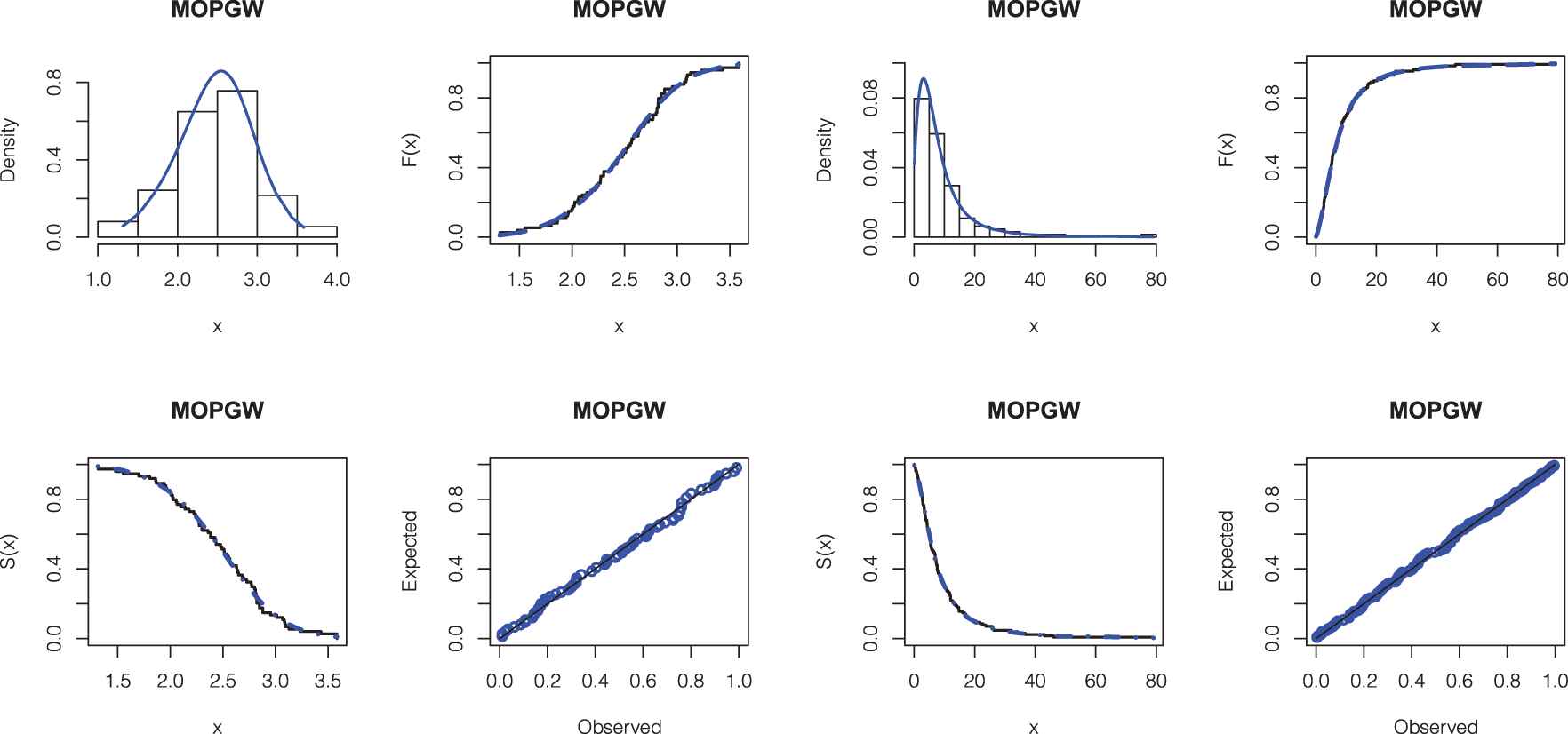
Fitted Marshall–Olkin power generalized Weibull (MOGPW) probability density function (PDF), estimated cumulative distribution function (CDF), SF, and PP plots (left panel) for gauge lengths data and (right panel) for cancer data.
The TTT plot of gauge lengths data and the HRF plot of the MOPGW distribution are displayed in Figure 4, whereas the TTT plot of cancer data and MOPGW HRF plot are shown in Figure 5. It is clear that the MOPGW HRF is increasing for gauge lengths data, whereas it is unimodal (upside down bathtub) for cancer data. Furthermore, the scaled TTT plot for gauge lengths data is concave which indicates an increasing HRF, whereas it is concave then convex for cancer data which indicates a unimodal HRF. Hence, the MOPGW distribution is a suitable for modeling both data sets.
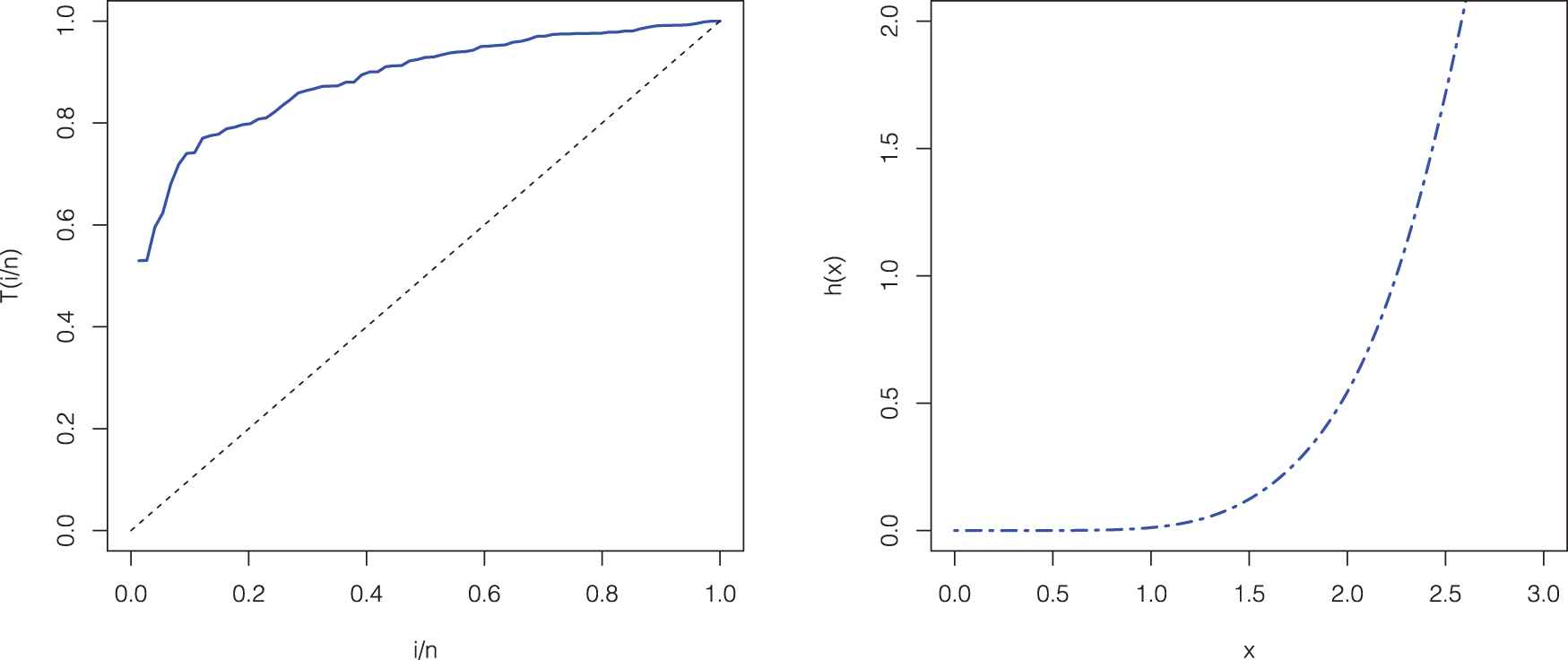
TTT plot for gauge lengths data (left panel) and the Marshall–Olkin power generalized Weibull (MOPGW) hazard rate function (HRF) plot (right panel).
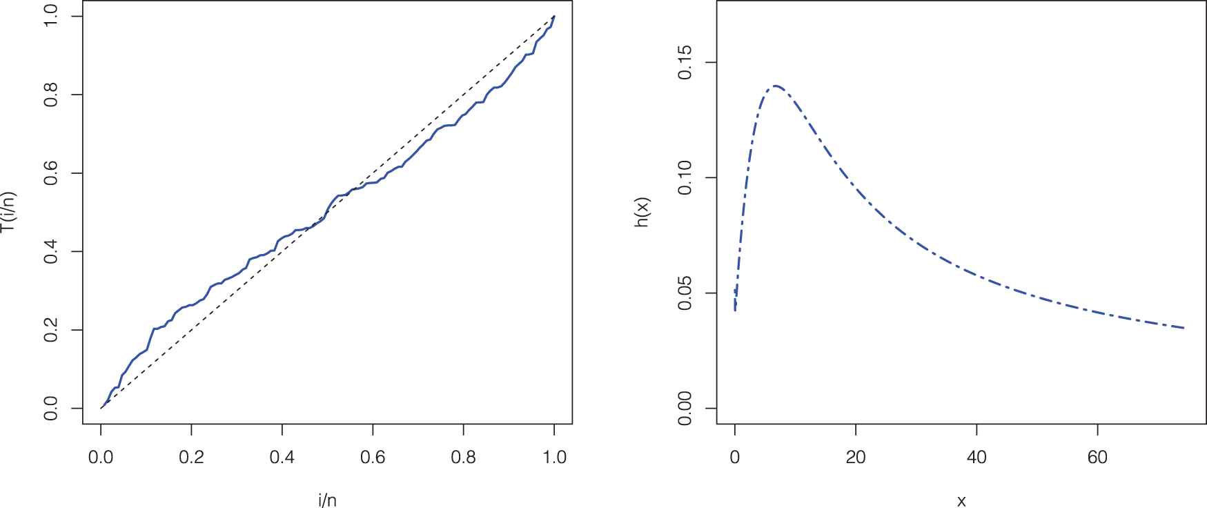
TTT plot for cancer data (left panel) and the Marshall–Olkin power generalized Weibull (MOPGW) hazard rate function (HRF) plot (right panel).
6. CONCLUSIONS
We propose and study the flexible four-parameter Marshall–Olkin power generalized Weibull (MOPGW) distribution. Some mathematical quantities of the MOPGW distributions are derived in explicit expressions. The maximum likelihood is utilized to estimate the MOPGW parameters and the simulation results show its performance. The MOPGW distribution can provide better fits than some other generalized extensions of the Weibull model for two real data sets from the engineering and medicine fields.
CONFLICT OF INTEREST
The authors declare no potential conflict of interests.
AUTHORS' CONTRIBUTIONS
All authors contributes equally.
ACKNOWLEDGMENTS
The authors would like to thank the editor and the reviewer for their constructive comments and suggestions which greatly improved the paper.
REFERENCES
Cite this article
TY  - JOUR
AU  - Ahmed Z. Afify
AU  - Devendra Kumar
AU  - I. Elbatal
PY  - 2020
DA  - 2020/05/21
TI  - Marshall–Olkin Power Generalized Weibull Distribution with Applications in Engineering and Medicine
JO  - Journal of Statistical Theory and Applications
SP  - 223
EP  - 237
VL  - 19
IS  - 2
SN  - 2214-1766
UR  - https://doi.org/10.2991/jsta.d.200507.004
DO  - 10.2991/jsta.d.200507.004
ID  - Afify2020
ER  -