Hjorth model; Generalized distribution family; Regression; Residual analysis; Characterizations; Bathtub; Hazard rate; PISA data; Student cognitive skill data
Abstract
We introduce a new flexible class of continuous distributions via the Hjorth's IDB model. We provide some mathematical properties of the new family. Characterizations based on two truncated moments, conditional expectation as well as in terms of the hazard function are presented. The maximum likelihood method is used for estimating the model parameters. We assess the performance of the maximum likelihood estimators in terms of biases and mean squared errors by means of the simulation study. A new regression model as well as residual analysis are presented. Finally, the usefulness of the family is illustrated by means of four real data sets. The new model provides consistently better fits than other competitive models for these data sets.
Hjorth [1] obtained a three-parameter distribution generalizing Rayleigh, exponential and linear failure rate distributions. Its cumulative distribution function (cdf) and probability density function (pdf) are given by
HHjx;α,β,θ=1−1+βx−θ∕βexp−αx2∕2,x≥0,(1)
and
hHjx;α,β,θ=αx1+βx+θ1+βx−θ∕β+1exp−αx2∕2,x>0,
respectively, where α>0 is the scale parameter and β,θ>0 are the shape parameters. Clearly, this distribution is reduced to Rayleigh, exponential and linear failure rate distributions for θ=0, α=β=0 and β=0, respectively. Since this distribution has increasing α≥θβ, decreasing α=0, constant α=β=0 and bathtub-shaped 0<α<βθ hazard rate functions (hrfs), it has also been named increasing-decresing-bathtub (IDB) distribution by the author. The quantile function (qf), denoted by Q(u), of the IDB distribution is the solution of the following equation:
1−u1+βQuθ∕β−exp−α2Qu2=0,u∈0,1.(2)
Hence, If U is a uniform random variable on (0,1) then QHjU is an IDB random variable, where QHj⋅ is the solution of the Equation (2). On the other hand, Alzaatreh et al. [2] proposed a new technique to construct wider families by using any pdf as a generator. This generator called the T-X family of distributions has cdf defined by
Fx=∫aWGx;ξrtdt,
where r(t) is the pdf of the random variable T∈a,b for −∞<a<b<∞ and WGx;ξ is a function of the baseline cdf which satisfies the following conditions: i) WGx;ξ∈a,b, ii) WGx;ξ is the differentiable and monotonically non-decreasing, iii) limx→−∞WGx;ξ=a and limx→∞WGx;ξ=b. The pdf of the T-X family is given by
fx=∂∂xWGx;ξrWGx;ξ.
Based on the above transformer T-X generator, we propose a new wider family of continuous distribution, the Hjorth-G family by replacing rt with the Hjorth density function and having cdf given by
where G¯x;ξ=1−Gx;ξ is the baseline survival function depending on a q×1 vector ξ of unknown parameters, Gx;ξ is the baseline cdf and α,β and θ are the extra scale and shape parameters which are ensure flexibility to baseline distribution. The pdf corresponding to equation (3) is given by
Hereafter, the random variable X with pdf (4) is denoted by X~ Hj −G(α,β,θ,ξ). Further, we can omit the dependence on the parameter vector ξ of the parameters and simply write Gx;ξ=Gx and gx;ξ=gx. If T is an IDB random variable with cdf (1), then X=G−11−e−T is the Hj-G random variable where G−1⋅ is the qf of the baseline distribution. Hence, qf of X is the solution of the non-linear equation G−11−e−QHju,u∈0,1. The hazard rate function (hrf) of X is given by
hx=gxαβlogG¯x−1logG¯x+θG¯x1−βlogG¯x.(5)
The goal of this work is to introduce a new flexible and wider family of the distributions based on T-X family using the IDB model. We are motivated to introduce the Hj −G family because it exhibits increasing, decreasing, constant, upside down, unimodal then bathtub as well as bathtub hazard rates as shown in Figures 1 and 2. The members of the Hj −G family can also be viewed as a suitable model for fitting the bimodal, unimodal, U-shaped and other shaped data. The Hj −G family outperforms several of the well-known lifetime distributions with respect to three real data applications as illustrated in Section 9. The new log- regression model based on the Hj – Weibull provides better fits than the log-Topp-Leone odd log-logistic-Weibull [3] and log-Weibull regression models for Stanford heart transplant data set.
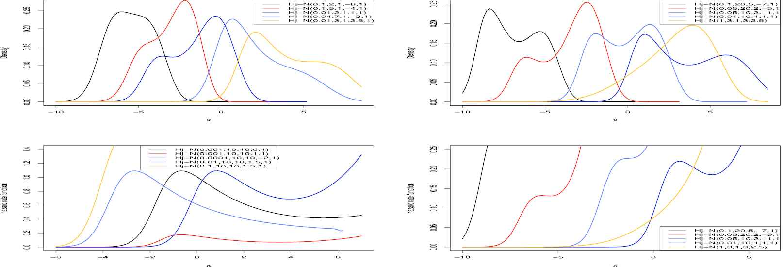
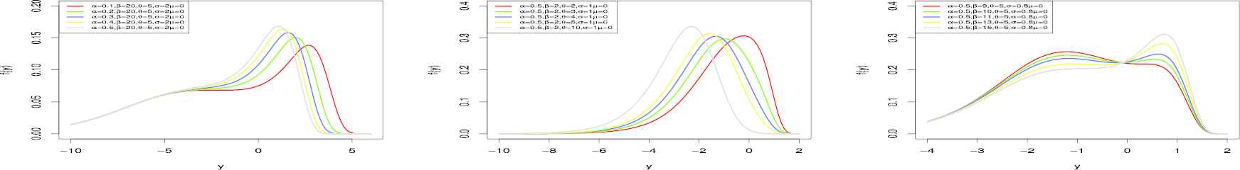
Figure 1
The probability density function (pdf) and hazard rate functions (hrf) of the Hj-Normal (Hj-N) distribution for selected parameter values.
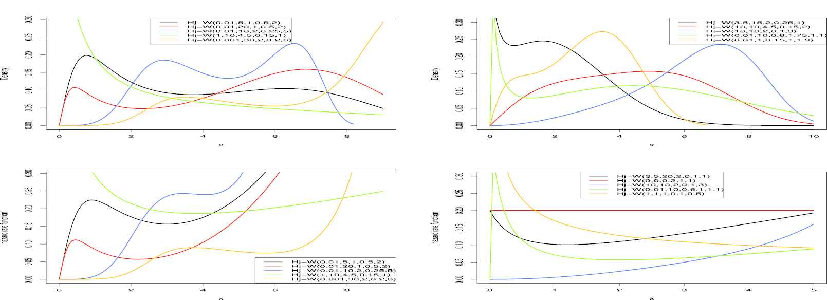
Figure 2
The probability density function (pdf) and hazard rate functions (hrf) of the Hj-Weibull (Hj-W) distribution for selected parameter values.
The paper is organized as follows: Some sub-families of the new family are introduced in Section 2. In Section 3, the series expansions for cdf and pdf of the new family are presented. In Section 4, some of its mathematical properties are derived. Section 5 deals with some characterizations of the new family. In Section 6, the maximum likelihood method is used to estimate the parameters. A new regression model as well as residual analysis are presented in Section 7. In Section 8, two simulation studies are performed to evaluate the efficiency of the maximum likelihood estimates. In Section 9, we illustrate the importance of the new family by means of three applications to real data sets. The paper is concluded in Section 10.
2. SPECIAL HJ-G DISTRIBUTIONS
The Hj-G family can extend to any baseline distribution due to its shape and scale parameters. So, the pdf (4) will generate more flexible distributions than baseline model. Also, Hj-G family includes some sub-families such as Rayleigh-G, exponential-G and linear failure rate-G families for θ=0, α=β=0 and β=0, respectively. We note that the Rayleigh-G and exponential-G families are the special members of the Weibull-G family which was introduced by Corderio et al. [4]. Here, we obtain three special models of the Hj-G family. These special models extend some well-known distributions given in the literature.
2.1. The Hj-Normal (Hj-N) Distribution
The normal distribution is very useful model in statistics and related field. Since, it has increasing hrf shape, symmetrical and uni-modal pdf shape, its data modeling area can be limited. To extend the normal distribution, we consider Hj-N distribution as our first example by taking Gx;μ,σ=Φx−μσ and gx;μ,σ=σ−1ϕx−μσ, the cdf and pdf, respectively, where x,μ∈ℝ, σ>0 and ϕ⋅ and Φ⋅ are the pdf and cdf of the standard normal distribution, respectively. We denote this distribution with Hj-N (α,β,θ,μ,σ). Some plots of the Hj-N density and hrf for selected parameter values are displayed in Figure 1. W note that the pdf shapes of the Hj-N can be skewed, bi-modal and uni-modal. Also, its hrf shapes are increasing and firstly increasing shape then bathtube shape.
2.2. The Hj-Weibull (Hj-W) Distribution
As our second example, we consider the Weibull distribution, which has monotone hrf and decreasing and uni-modal pdf, with shape parameter γ>0 and scale parameter λ>0. Its cdf and pdf are given by Gx;γ,λ=1−exp−(λx)γ and gx;γ,λ=λγx(γ−1)exp−(λx)γ for x>0, respectively. We denote this distribution with Hj-W (α,β,θ,λ,γ). Some plots of the Hj-W density and hrf for selected parameter values are displayed in Figure 2. Figure 2 shows that the pdf and hrf shapes of the Hj-W can be very flexible. For example, the new extended Weibull distribution has bi-modal, uni-modal, decreasing, firstly increasing shape then U shaped pdf. Nevertheless, it has both monotone and non-monotone hrf shape such as bathtube shape and firstly increasing shape then bathtube shape.
2.3. The Hj-Uniform (Hj-U) Distribution
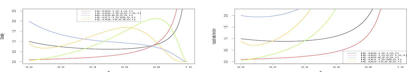
As our third example, let the baseline distribution have an uniform distribution in the interval a,b Then Gx;a,b=(x−a)∕(b−a) and gx;a,b=1∕(b−a) for a<x<b, a,b∈ℝ. We denote this distribution with Hj-U (α,β,θ,a,b). Some plots of the Hj-U density and hrf for selected parameter values are displayed in Figure 3. Figure 3 shows that the pdf can be increasing, decreasing, uni-modal, firstly decresing then uni-modal and U-shaped. Its hrf has increasing and bathtube shape. Hence, Hj-U distribution may be suggested for hrf model with bathtube shape.
Figure 3
The probability density function (pdf) and hazard rate functions (hrf) of the Hj-Uniform (Hj-U) distribution for selected parameter values.
3. USEFUL EXPANSIONS
In this section, we provide a useful linear representation of the Hj-G cdf function
Fx=1−exp−α2−log1−Gx2︸Ai1−βlog1−Gx−θ∕β.
Expanding the quantity Ai in power series, we can write
Fx=1−∑i=0∞−13ilog1−Gx2ii!−1α∕2i1−βlog1−Gx−θ∕β︸Bi,
and expanding the quantity Bi by via Taylor series
τζ=∑j=0∞j!−1τ−1jζj,
where j is a positive integer and ζj=ζζ−1…ζ−j+1 is the descending factorial, we get
where υk+1=−vk+1 and πk+1x=k+1gxGxk denotes the exp-G class density with power parameter k+1.
4. SOME PROPERTIES OF THE HJ-G FAMILY
4.1. General Properties
The rth ordinary moment of X is given by μr′=E(Xr)=∫−∞∞xrfxdx. Then, we obtain μr′=∑k=0∞υk+1E(Yk+1r), where Yγr=γ∫−∞∞xrGxγ−1gxdx, which can be computed numerically in terms of the baseline quantile function (qf) QG(u;ξ)=G−1(x;ξ) as E(Yαn)=α∫01uα−1QG(u;ξ)ndu. by setting r=1 in μr′, we have the mean of X. The last integration can be computed numerically for most parent distributions. The rth central moment of X, say μn, follows as μr=E(X−μ1′)n=∑h=0n(−1)hnh(μ1′)nμn−h′. For the skedwness and kurtosis coefficients, we have β1=μ32μ23andβ2=μ4μ22. The values for mean, variance, β1 and β2 for selected Hj-W distributions are shown in Table 1. Table 1 shows that Hj-N distribution can be left skewed and right skewed as well as having different kurtosis values. Hence, the Hj-W model can be useful for data modeling in terms of skewness and kurtosis.
(α,β,θ,λ,γ)
μ1′
Variance
β1
β2
(0.5, 0.5, 0.5, 0.5, 0.5)
4.4975
37.1694
2.6572
13.5148
(1, 1, 1, 1, 1)
0.7706
0.3715
1.0395
3.9265
(2, 2, 0.5, 1, 2)
0.8161
0.0849
−0.1659
2.6427
(5, 5, 5, 5, 5)
0.1385
0.0011
−0.3015
2.6162
(0.5, 2, 0.5, 2, 0.5)
1.4083
3.1419
2.3539
11.1339
(1, 2, 3, 4, 5)
0.1918
0.0022
−0.1629
2.6292
(5, 4, 3, 2, 1)
0.1626
0.0188
1.1156
4.0671
(5, 10, 15, 20, 25)
0.0444
0.00001
−27.0075
31116
Table 1
Mean, variance, coefficients of skewness and kurtosis for Hj-Weibull (Hj-W) distributions.
The nth descending factorial moment of X (for n=1,2,…) is
μn′=E[X(n)]=EXX−1×…×X−n+1=∑k=0nsn,kμk′,
where s(n,k)=(k!)−1[dkk(n)/dxk]x=0 is the Stirling number of the first kind. Here, we provide two formulae for the moment generating function (mgf) MXt=EetX of X. Clearly, the first one can be derived from Equation (7) as MXt=∑k=0∞υk+1Mk+1t, where Mkt is the mgf of Yk+1. Hence, MXt can be determined from the exp-G generating function. A second formula for MXt follows from (7) as MXt=∑j=0∞υk+1τt,k, where τt,k=∫01exptQGuukdu and QG(u) is the qf corresponding to Gx;ξ, i.e., QG(u)=G−1(u;ξ). The rth incomplete moment of X is defined by mr(y)=∫−∞yxrf(x)dx. From (7) we can write mr(y)=∑k=0∞υk+1mr,k(y), where mr,γ(y)=E(Yγr)=∫0Gy;ξQGru;ξuγ−1du. The integral mr,γ(y) can be determined analytically for special models with closed-form expressions for QG(u;ξ) or computed at least numerically for most baseline distributions.
4.2. Order Statistics
Suppose X1,…,Xn is a random sample from any Hj-G distribution. Let Xi:n denote the ith order statistic. The pdf of Xi:n can be expressed as
and υr+1 is given in Section 3 and the quantities fj+i−1,k can be determined with fj+i−1,0=c0j+i−1 and recursively for k≥1, fj+i−1,k=kc0−1∑m=1k[m(j+i)−k]cmfj+i−1,k−m. Equation (8) is the main result of this section. It reveals that the pdf of the Hj-G order statistics is a linear combination of Exp-G density functions. So, several mathematical quantities of the Hj-G-G order statistics such as ordinary, incomplete and factorial moments, mean deviations and several others can be determined from those quantities of the exp-G distribution.
5. CHARACTERIZATION
This section deals with various characterizations of the Hj-G distribution. These characterizations are based on i a simple relationship between two truncated moments; ii the hazard function and iii conditional expectation of a function of the random variable. It should be mentioned that for characterization i the cdf is not required to have a closed form. We present our characterizations i−iii in three subsections.
5.1. Characterizations Based on Two Truncated Moments
In this subsection we present characterizations of Hj-G distribution in terms of a simple relationship between two truncated moments. The first characterization result employs a theorem due to Glänzel [7] see Theorem 5.1.1 below. Note that the result holds also when the interval H is not closed. Moreover, as mentioned above, it could be also applied when the cdf F does not have a closed form. As shown in Glänzel [8], this characterization is stable in the sense of weak convergence.
Theorem 5.1.1.
LetΩ,ℱ,Pbe a given probability space and letH=d,ebe an interval for somed<e (d=−∞,e=∞might as well be allowed). LetX:Ω→Hbe a continuous random variable with the distribution functionFand letq1andq2be two real functions defined onHsuch that
Eq2X|X≥x=Eq1X|X≥xηx,x∈H,
is defined with some real functionη. Assume thatq1,q2∈C1H, η∈C2HandFis twice continuously differentiable and strictly monotone function on the setH. Finally, assume that the equationηq1=q2has no real solution in the interior ofH. ThenFis uniquely determined by the functionsq1,q2andη, particularly
Fx=∫axCη′uηuq1u−q2uexp−sudu,
where the functions is a solution of the differential equations′=η′q1ηq1−q2andCis the normalization constant, such that∫HdF=1.
Proposition 5.1.1.
LetX:Ω→ℝbe a continuous random variable and let, q1x=−logG¯x1−βlogG¯xθβ+1αβlogG¯x−1logG¯x+θandq2x=q1xexp−α2logG¯x2forx∈ℝ. The random variableXhas pdf (4) if and only if the functionηdefined in Theorem 5.1.1 has the form
LetX:Ω→ℝbe a continuous random variable and letq1xbe as in Proposition 5.1.1. The pdf ofXis (4) if and only if there exist functionsq2andηdefined in Theorem 5.1.1 satisfying the differential equation
η′xq1xηxq1x−q2x=−αgxlogG¯xG¯xx∈ℝ.
The general solution of the differential equation in Corollary 5.1.1 is
whereDis a constant. Note that a set of functions satisfying the above differential equation is given in Proposition 5.1.1 withD=0. However, it should be also noted that there are other tripletsq1,q2,ηsatisfying the conditions of Theorem 5.1.1.
5.2. Characterization Based on Hazard Function
It is known that the hazard function, hF, of a twice differentiable distribution function, F, satisfies the first order differential equation
f′(x)f(x)=hF′(x)hF(x)−hF(x).
For many univariate continuous distributions, this is the only characterization available in terms of the hazard function. The following characterization establishes a non-trivial characterization of Hj-G distribution in terms of the hazard function, which is not of the above trivial form.
Proposition 5.2.1.
LetX:Ω→ℝbe a continuous random variable. The pdf ofXis (4) if and only if its hazard functionhFxsatisfies the differential equation
If X has pdf (4), then clearly the above differential equation holds. Now, if the differential equation holds, then
ddxgx−1hFx=ddxαβlogG¯x−1logG¯x+θG¯x1−βlogG¯x,
or
hFx=gxαβlogG¯x−1logG¯x+θG¯x1−βlogG¯x,
which is the hazard function of the Hj-G distribution.
5.3. Characterizations Based on Conditional Expectation
The following proposition has already appeared in Hamedani [9], so we will just state it here which can be used to characterize the Hj-G distribution.
Proposition 5.3.1.
LetX:Ω→a,bbe a continuous random variable withcdfF. Letψxbe a differentiable function ona,bwithlimx→a+ψx=1. Then forδ≠1,
EψX|X≥x=δψx,x∈a,b,
if and only if
ψx=1−Fx1δ−1,x∈a,b.
Remark 5.3.1
(a) For ψx=exp−logG¯x21−βlogG¯x2θαβ, δ=α2+α and a,b=ℝ, Proposition 5.3.1 provides a characterization of Hj-G distribution. (b) Of course there are other suitable functions than the one we mentioned above, which is chosen for simplicity.
6. MAXIMUM LIKELIHOOD ESTIMATION (MLE)
We consider the estimation of the unknown parameters of the new family from complete samples only by maximum likelihood method. Let x1,⋯,xn be a random sample from the Hj-G family with a (q+3)×1 parameter vector Θ=(α,β,θ,ξ⊺)⊺, where ξ is a q×1 baseline parameter vector. The log-likelihood function for Θ is given by
Setting the nonlinear system of equations Uα=Uβ=Uθ=Uξr=0 (for r=1,…,q) and solving them simultaneously yields the MLEs Θ^=(α^,β^,θ^,ξ^⊺)⊺. To solve these equations, it is more convenient to use nonlinear optimization methods such as the quasi-Newton algorithm to numerically maximize ℓ(Θ). For interval estimation of the parameters, we can evaluate numerically the elements of the (q+3)×(q+3) observed information matrix J(Θ)={−∂2ℓ∂θrθs}. Under the standard regularity conditions, when n→∞, the distribution of Θ^ can be approximated by a multivariate normal Np(0,J(Θ^)−1) distribution to construct approximate confidence intervals for the parameters. Here, J(Θ^) is the total observed information matrix evaluated at Θ^. The method of the re-sampling bootstrap can be used for correcting the biases of the MLEs of the model parameters. Good interval estimates may also be obtained using the bootstrap percentile method.
7. SIMULATION STUDY
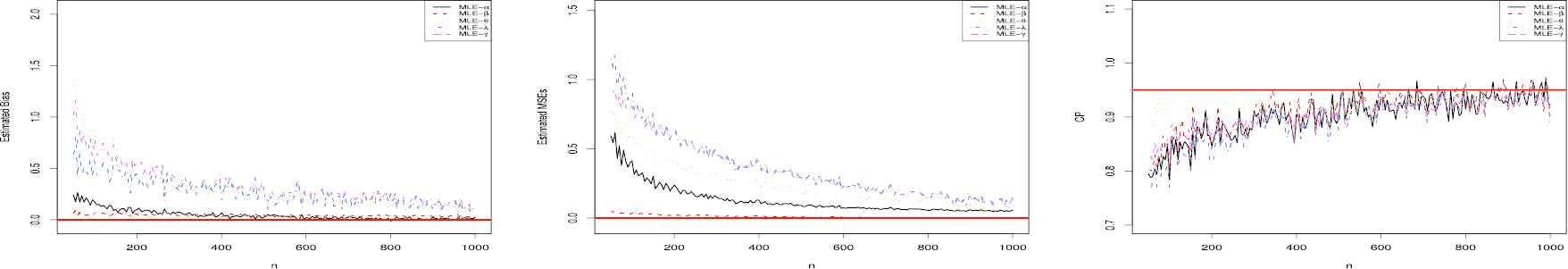
In this section, the performance of the MLEs of Hj-W distribution is discussed via simulation study. The inverse transform method is used to generate random variables from Hj-W distribution. The performance of the MLEs is evaluated based on the following measures: biases, mean square error (MSE) and coverage probability (CP). N=1,000 samples of sizes n=50,55,…,1000 is generated from the Hj-W distribution with α=0.5,β=0.5,θ=2,λ=2,γ=3. The MLEs of the model parameters are obtained for each generated sample, say (αi^,βi^,θi^,λi^,γi^), for i=1,…,N. The standard errors of the MLEs are evaluated by inverting the observed information matrix, namely (sαî,sβî,sθî,sλî,sγî) for i=1,…,N. The estimated biases and MSEs and CPs are given by Bias^ε(n)=1N∑i=1N(ε^i−ε), MSE^ε(n)=1N∑i=1N(ε^i−ε)2, and CPε(n)=1N∑i=1NI(ε^i−1.95996sε^i,ε^i+1.95996sε^i) where ε=α,β,θ,λ,γ and sεî is standard error of ε̂i for each generated sample.
Figure 4 displays the simulation results for above measures. As seen from Figure 4, the estimated biases and MSEs approach zero when the sample size increases. As expected, CPs are near the nominal value (0.95) for sufficiently large sample sizes. The simulation results verify the consistency property of MLE. The similar results can be obtained for different parameter vector.
Figure 4
Estimated coverage probability (CPs), biases and mean square errors (MSEs) for the selected parameter vector.
8. LOG-HJ-W REGRESSION MODEL
Consider the Hj-W distribution with five parameters presented in Subsection 2.2. Henceforth, X denotes a random variable following the Hj-W distribution and Y=log(X). The density function of Y (for y∈ℝ) obtained by replacing γ=1∕σ and λ=1∕expμ, can be expressed as
where μ∈ℝ is the location parameter, σ>0 is the scale parameter and α>0, β>0 and θ>0 are the shape parameters. We refer to equation (9) as the log-Hj-W (LHj-W) distribution, say Y~LHj-W(α,β,θ,μ,σ). Figure 5 provides some plots of the density function (9) for selected parameter values. They reveal that this distribution is a good candidate for modeling left skewed and bimodal data sets.
Figure 5
Plots of the LHj-W density function for some parameter values.
The survival function corresponding to (9) is given by
Based on the LHj-W density, we propose a linear location-scale regression model linking the response variable yi and to explanatory variable vector viT=vi1,…,vip given by
yi=viTβ+σzi,i=1,…,n(12)
where the random error zi has the density function (11), β=(β1,…,βp)T, σ>0, α>0, β>0 and θ>0 are unknown parameters. The parameter μi=viTβ is the location of yi. The location parameter vector μ=(μ1,…,μn)T is represented by a linear model μ=Vβ, where V=(v1,…,vn)T is a known model matrix. Consider a sample (y1,v1),…,(yn,vn) of n independent observations, where each random response is defined by yi=min{log(xi),log(ci)}. We assume non-informative censoring such that the observed lifetimes and censoring times are independent. Let F and C be the sets of individuals for which yi is the log-lifetime or log-censoring, respectively. The log-likelihood function for the vector of parameters τ=(α,β,θ,σ,βT)T from model (12) has the form l(τ)=∑i∈Fli(τ)+∑i∈Cli(c)(τ), where li(τ)=log[f(yi)], li(c)(τ)=log[S(yi)], f(yi) is the density (9) and S(yi) is the survival function (10) of Yi. The total log-likelihood function for τ is given by
where ui=exp(zi), zi=(yi−μi)∕σi, and r is the number of uncensored observations (failures). The MLE τ^ of the vector of unknown parameters can be obtained by maximizing the log-likelihood function (13). The R software is used to estimate τ^.
8.1. Residual Analysis
Residual analysis has critical role in checking the adequacy of the fitted model. In order to analyze departures from the error assumption, two types of residuals are considered: martingale and modified deviance residuals.
8.1.1. Martingale Residual
The martingale residuals is defined in counting process and takes values between +1 and −∞ (see [10] for details). The martingale residuals for LHj-W model is
The main drawback of the martingale residual is that when the fitted model is correct, it is not symmetrically distributed about zero. To overcome this problem, modified deviance residual was proposed by Therneau et al. [11]. Th modified deviance residual for LHj-W model is
In this section, we consider three applications to real data sets to show the modeling ability of the Hj-N, Hj-W and Hj-U distributions. We compare these distribution models with both distributions of some members of the T-X family, where W[G(x)] is equal to −log[1−G(x)], and some generalizations of ordinary normal, Weibull and uniform distributions. These families and generalized models are the Mc Donald-G (Mc-G) family [12], Gompertz-G (Gom-G) family [13], Generalized odd log logistic-G (GOLL-G) family [14], Weibull-G (W-G) family [4], Lomax-G (Lx-G) family [15], Lindley-G (Li-G) family [16], logistic-G (L-G) family [17], Kumaraswamy odd log logistic normal (KwOLLN) distribution [18], odd Burr normal (OBN) distribution [19], Zografos-Balakkrishnan odd log logistic Weibull (ZBOLLW) distribution [20], additive Weibull (AW) distribution [21] and gamma uniform (GU) distribution [22]. The cdfs of these distributions are available in the literature. To determine the best model, we also compute the estimated log-likelihood values ℓ̂, Akaike Information Criteria (AIC), corrected Akaike information criterion (CAIC), Bayesian information criterion (BIC), Hannan–Quinn information criterion (HQIC), Cramer-von-Mises (W∗) and Anderson-Darling (A∗) goodness of-fit statistics for all distribution models. We note that the statistics W∗ and A∗ are described in detail in [23]. In general, it can be chosen as the best model the one which has the smaller the values of the AIC, CAIC, BIC, HQIC, W∗ and A∗ statistics and the larger the values of ℓ̂ and p-values. All computations are performed by the maxLik routine in the R programme. The details are given below.
9.1. Otis IQ Scores of Non-White Males Data Set
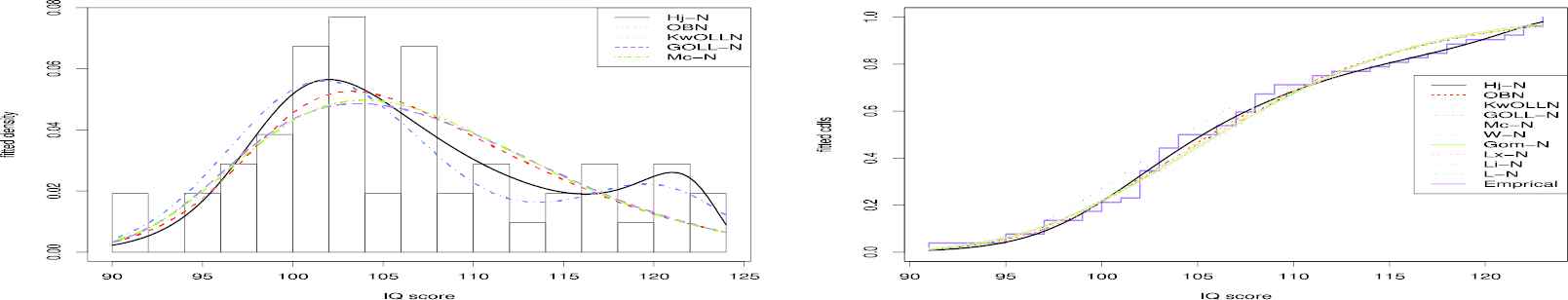
The first real data set is the data on the Otis IQ Scores of 52 non-white males hired by a large insurance company in 1971. This data set has been analyzed by [24–26] and [27]. On the data set, we compare the Hj-N model with Mc-N, Lx-N, W-N, KwOLLN, L-N, OBN, GOLL-N, Gom-N and Li-N models. Table 2 shows MLEs and standard erros of the estimates for the first dat set. Table 3 lists information criteria results and goodness-of-fits statistics. Table 3 clearly show that the Hj-N model has the smallest values AIC, CAIC, BIC, HQIC, W∗ and A∗ statistics and it has the largest values for ℓ̂ and two p-values among the fitted models. So, it can be chosen as the best model based on these criteria. For this data set, the plots of the fitted pdfs and cdfs for all models are shown in Figure 6. From this figure, we see that the Hj-N, Mc-N and KwOLLN models fit data as bi-modal shape whereas the OBN model fits data as uni-modal shape.
Data Set
Model
α̂
β̂
θ̂
μ̂
σ̂
I
Hj-N
190,363.1425
518,889.4549
152,083.8273
154.4301
11.9168
(5.9316)
(380.4220)
(380.4954)
(0.00001)
(0.0862)
KwOLLN
5.8735
84.4204
0.0221
113.0728
2.0037
(0.2310)
(6.8585)
(0.0026)
(0.0308)
(0.0519)
Mc-N
0.0160
0.0573
2.7977
111.0082
1.4883
(0.0023)
(0.0132)
(0.0315)
(0.0001)
(0.0001)
GOLL-N
0.7348
-
18.6911
84.2008
12.0843
(0.1867)
(6.8108)
(4.7654)
(2.2345)
OBN
1.7777
-
0.2647
98.9947
7.7191
(0.8162)
(0.1183)
(1.9371)
(2.6981)
W-N
0.1546
-
0.9030
96.8421
3.5746
(0.0432)
(0.0972)
(0.0002)
(0.0002)
Gom-N
0.0020
-
0.0921
94.9562
3.4364
(0.0152)
(0.0196)
(0.0007)
(0.0007)
Lx-N
118.0650
376.2148
-
99.5811
5.4795
(93.3838)
(92.8438)
(1.0954)
(0.4381)
Li-N
−
-
0.1470
90.5867
4.0007
(0.0144)
(0.0001)
(0.0001)
L-N
−
-
2.5576
101.6204
12.0705
(0.9339)
(1.7310)
(4.3032)
Table 2
MLEs and standard erros of the estimates (in parentheses) for the first data set.
Data Set
Model
AIC
CAIC
BIC
HQIC
A∗
W∗
−ℓ^
I
Hj-N
366.8823
368.1866
376.6385
370.6226
0.2925
0.0428
178.4411
[0.9434]
{0.9198}
KwOLLN
368.0000
369.3043
377.7562
371.7403
0.3144
0.0446
179.0001
[0.9266]
{0.9098}
Mc-N
368.4839
369.7883
378.2401
372.2242
0.3422
0.0520
179.2420
[0.9028]
{0.9030}
GOLL-N
372.5455
373.3966
380.3505
375.5378
0.4404
0.0683
182.2728
[0.8072]
{0.7639}
OBN
371.8735
372.7245
379.6784
374.8657
0.3973
0.0584
181.9367
[0.8508]
{0.8262}
W-N
372.5644
373.4154
380.3693
375.5566
0.4698
0.0750
182.2822
[0.7770]
{0.7231}
Gom-N
371.0419
371.8929
378.8468
374.0341
0.5295
0.0856
181.5209
[0.7160]
{0.6616}
Lx-N
373.2565
374.1076
381.0615
376.2488
0.6205
0.1031
182.6283
[0.6280]
{0.5715}
Li-N
370.9549
371.4549
376.8087
373.1991
0.7868
0.1486
182.4775
[0.4900]
{0.3947}
L-N
372.8924
373.3924
378.7461
375.1365
0.4423
0.0639
183.4462
[0.8053]
{0.7911}
Table 3
Information criteria results, A∗, W∗ and ℓ̂ statistics ([⋅] and {⋅} denote their p-values) for the first data set.
Figure 6
The fitted probability density functions (pdfs) and cumulative distribution functions (cdfs) for the first data set.
9.2. Failure Times Data Set
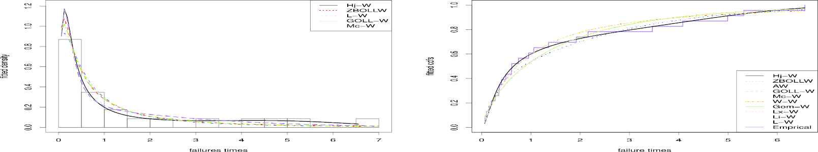
The second data set represents the times between successive failures (in thousands of hours) in events of secondary reactor pumps studied by [28,29] and [30]. This data set is also known as bathtub shaped. So, for this data set, we compare the Hj-W model with AW, Mc-W, Lx-W, W-W, ZBOLLW, L-W, GOLL-W, Gom-W and Li-W models. We fitted the Hj model and obtained its ℓ̂ value as −31.2520. Table 4 shows MLEs and standard erros of the estimates for the second data set. Table 5 lists information criteria results and goodness-of-fits statistics. The Hj-W model has the smallest values of the AIC, HQIC, W∗ and A∗ statistics and have the largest values for ℓ̂ and all p-values among the fitted models. For this data set, the plots of the fitted pdfs and cdfs for all models are shown in Figure 7. From this figure, we see that the Hj-W model fits the histograms of the data sets with more adequate fitting than Li-W and other models.
Data Set
Model
α̂
β̂
θ̂
λ̂
γ̂
II
Hj-W
0.0031
23.3597
6.9156
0.9910
1.8949
(0.0018)
(6.5439)
(2.1775)
(0.0152)
(0.0007)
ZBOLLW
2.5977
6.2815
-
41.9548
0.2567
(3.3552)
(4.1634)
(12.3595)
(0.1468)
Mc-W
87.0504
119.6097
2.3397
37.5696
0.0487
(4.2657)
(1.4467)
(0.1265)
(2.5664)
(0.0064)
GOLL-W
0.2619
-
10.3956
4.1457
0.8139
(0.0579)
(0.2475)
(0.0893)
(0.7005)
W-W
0.1100
-
1.1545
11.0445
0.6995
(0.0523)
(0.1856)
(0.0051)
(0.0001)
Gom-W
0.0023
-
0.0912
15.1874
0.7808
(0.0230)
(0.0294)
(0.0003)
(0.0001)
Lx-W
48.4187
99.9372
-
1.7814
0.8161
(11.7869)
(17.9206)
(1.0382)
(0.1314)
Li-W
−
-
27.1223
0.0126
0.1298
(10.4406)
(0.0099)
(0.1298)
L-W
−
-
21.5282
1.4143
0.0571
(9.5853)
(0.4227)
(0.0272)
AW
0.1576
11.1873
-
0.6779
0.7575
(0.0172)
(10.4301)
(0.2075)
(0.1372)
Table 4
MLEs and standard erros of the estimates (in parentheses) for the second data set.
Data Set
Model
AIC
CAIC
BIC
HQIC
A∗
W∗
−ℓ^
II
Hj-W
68.7731
72.3025
74.4506
70.2010
0.1295
0.0157
29.3865
[0.9997]
{0.9996}
ZBOLL-W
71.1057
73.3279
75.6476
72.2480
0.2213
0.0243
31.5528
[0.9835]
{0.9923}
Mc-W
73.5915
77.1209
79.2690
75.0193
0.2264
0.0256
31.7957
[0.9814]
{0.9898}
GOLL-W
69.9227
72.1450
74.4647
71.0650
0.2400
0.0384
30.9614
[0.9754]
{0.9445}
W-W
73.0278
75.2500
77.5698
74.1701
0.4040
0.0617
32.5139
[0.8433]
{0.8076}
Gom-W
72.3346
74.5568
76.8766
73.4770
0.3845
0.0569
32.1673
[0.8626]
{0.8382}
Lx-W
73.0204
75.2427
77.5625
74.1628
0.3965
0.0602
32.5102
[0.8509]
{0.8175}
Li-W
71.0288
72.2920
74.4354
71.8855
0.4047
0.0619
32.5144
[0.8426]
{0.8066}
L-W
71.2273
72.4905
74.6338
72.0841
0.2326
0.0259
32.6136
[0.9788]
{0.9891}
AW
70.5462
72.7684
75.0881
71.6884
0.3730
0.0600
31.2731
[0.8738]
{0.8186}
Table 5
Information criteria results, A∗, W∗ and ℓ̂ statistics ([⋅] and {⋅} denote their p-values) for the second data set.
Figure 7
The fitted probability density functions (pdfs) and cumulative distribution functions (cdfs) for the second data set.
9.3. Student's Cognitive Skill Data
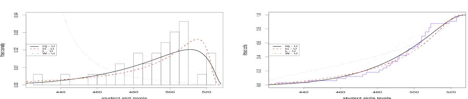
The third data set contains the student's cognitive skills for Organisation for Economic Co-operation and Development (OECD) countries. The score of student's cognitive skill represents the average score in reading, mathematics and science as assessed by the OECD's Programme for International Student Assessment (PISA). The data set can be found in https://stats.oecd.org/index.aspx?DataSetCode=BL. By using this data set, we compare the Hj-U model with GU, L-U and W-U models. We note that since a<x<b, the MLE of the a and b are the minumum order statistic x1:n and maximum order statistic xn:n respectively. Hence, we assume that the parameters are a=416 and b=529 for all fitted models. Table 6 shows MLEs and standard erros of the estimates for the third data set. Table 7 lists information criteria results and goodness-of-fits statistics. The Hj-U model has the smallest values of the AIC, CAIC, HQIC, W∗ and A∗ statistics and have the largest values of the ℓ̂ and all p-values among the fitted models. So, it can be chosen as the best model based on these criteria. For this data set, the plots of the fitted pdfs and cdfs for all models are shown in Figure 8. From this figure, The Hj-U model has fitted the data as uni-modal shaped.
Data Set
Model
α̂
β̂
θ̂
a
b
III
Hj-U
0.8393
11.0082
0.1020
416
529
(0.1537)
(4.2005)
(0.2336)
GU
1.0723
3.9112
-
416
529
(0.2339)
(1.0792)
L-U
2.7437
-
-
416
529
(0.4026)
W-U
0.4537
-
0.6334
416
529
(0.1032)
(0.0930)
Table 6
MLEs and standard erros of the estimates (in parentheses) for the third data set.
Data Set
Model
AIC
CAIC
BIC
HQIC
A∗
W∗
−ℓ^
III
Hj-U
295.7462
296.5738
300.2357
297.2568
0.6284
0.1031
144.8731
[0.6202]
{0.5726}
GU
297.7327
298.1327
300.7257
298.7398
1.2184
0.2049
146.8684
[0.2604]
{0.2588}
L-U
299.6478
299.7768
301.1443
300.1513
2.5881
0.5574
148.8239
[0.0449]
{0.0279}
W-U
404.1662
404.5662
407.1592
405.1733
2.8695
0.5562
200.0831
[0.0322]
{0.0281}
Table 7
Information criteria results, A∗, W∗ and ℓ̂ statistics ([⋅] and {⋅} denote their p-values) for the third data set.
Figure 8
The fitted probability density functions (pdfs) and cumulative distribution functions (cdfs) for the third data set.
Finally, when we observe all results, we can say that the Hj-N, Hj-W and Hj-U models could be chosen as the best models for the three data sets via the above criteria.
9.4. Stanford Heart Transplant Data
Recently, Brito et al. [3] introduced the Log-Topp-Leone odd log-logistic-Weibull (Log-TLOLL-W) regression model. Brito et al. [3] used the Stanford heart transplant data set to prove the usefulness of Log-TLOLL-W regression model. Here, we use the same data set to demonstrate the flexibility of LHj-W regression model against the Log-TLOLL-W and Log-Weibull regression models. These data set is available in p3state.msm package of R software. The sample size is n=103, the percentage of censored observations is 27%. The goal of this study is to relate the survival times t of patients with the following explanatory variables: x1- year of acceptance to the program; x2- age of patient (in years); x3- previous surgery status 1=yes,0=no; x4- transplant indicator 1=yes,0=no; ci - censoring indicator (0 = censoring, 1 = lifetime observed). The regression model fitted to the stanford heart transplant data is given by
yi=β0+β1xi1+β2xi2+β3xi3+β4xi4+σzi,
respectively, where the random variable yi follows the LHj-W distribution given in (9). The results for the above regression models are presented in Table 8. The MLEs of the model parameters and their SEs, p values and −ℓ, AIC and BIC statistics are listed in Table 8. Based on the figures in Table 8, LHj-W model has the lowest values of the −ℓ, AIC and BIC statistics. Therefore, it is clear that LHj-W regression model outperforms the others for this data set. In view of the results of LHj-W regression model, β0, β1 and β2 are statistically significant at 1% level.
Models
Log-Weibull
Log-TLOLL-W
LHj-W
Parameters
Estimate
S.E.
p-value
Estimate
S.E.
p-value
Estimate
S.E.
p-value
α
-
-
-
2.34
3.546
-
1.662
0.541
-
β
-
-
-
-
-
-
5.382
6.910
-
θ
-
-
-
24.029
3.015
-
19.326
12.172
-
σ
1.478
0.133
-
9.68
12.526
-
1.223
0.141
-
β0
1.639
6.835
0.811
−0.645
8.459
0.939
6.398
0.485
<0.001
β1
0.104
0.096
0.279
0.074
0.097
0.448
0.234
0.096
0.014
β2
−0.092
0.02
<0.001
−0.053
0.02
0.009
−0.066
0.018
<0.001
β3
1.126
0.658
0.087
1.676
0.597
0.005
0.139
0.512
0.785
β4
2.544
0.378
<0.001
2.394
0.384
<0.001
0.262
0.377
0.487
−ℓ
171.2405
164.684
160.061
AIC
354.481
345.368
338.122
BIC
370.2894
366.4458
361.834
Table 8
MLEs of the parameters to Stanford Heart Transplant Data for Log-Weibull, Log-TLOLL-W and LHj-W regression models with corresponding SEs, p-values and −ℓ, AIC and BIC statistics.
Finally, when we observe all results, we can say that the Hj-N, Hj-W and Hj-U models could be chosen as the best models for the three data sets via the above criteria.
9.4.1. Residual analysis of LHj-W model for Stanford heart transplant data set
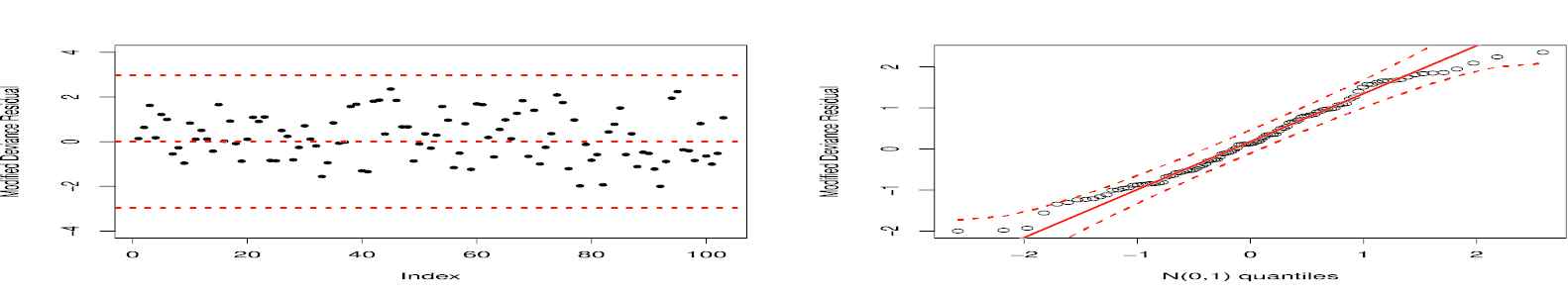
Figure 9 displays the index plot of the modified deviance residuals and its Q-Q plot against N(0,1) quantiles for Stanford heart transplant data set. Based on Figure 9, we conclude that none of observed values appear as possible outliers. Therefore, the fitted model is appropriate for this data set.
Figure 9
Index plot of the modified deviance residual (left) and Q-Q plot for modified deviance residual (right).
10. CONCLUSIONS
In this work, we introduce a new flexible class of continuous distributions via the Hjorth's IDB model. We provide some mathematical properties of the new family. Characterizations based on two truncated moments, conditional expectation as well as in terms of the hazard function are presented. The maximum likelihood method is used for estimating the model parameters. We assess the performance of the maximum likelihood estimators in terms of the biases and mean squared errors by means of two simulation studies. A new regression model as well as residual analysis are presented, Finally, the usefulness of the family is illustrated by means of three real data sets. The new model provides consistently better fits than other competitive models for these data sets.
9.G.G. Hamedani, On Certain Generalized Gamma Convolution Distributions II, Department of Mathematics, Statistics and Computer Science, Marquette University, Milwaukee, Wisconsin, USA, 2013. Technical Report No. 484
10.T.R. Fleming and D.P. Harrington, Counting Process and Survival Analysis, John Wiley, New York, NY, USA, 1994.
TY  - JOUR
AU  - Mustafa Ç. Korkmaz
AU  - Emrah Altun
AU  - Haitham M. Yousof
AU  - G. G. Hamedani
PY  - 2020
DA  - 2020/03/12
TI  - The Hjorth's IDB Generator of Distributions: Properties, Characterizations, Regression Modeling and Applications
JO  - Journal of Statistical Theory and Applications
SP  - 59
EP  - 74
VL  - 19
IS  - 1
SN  - 2214-1766
UR  - https://doi.org/10.2991/jsta.d.200302.001
DO  - 10.2991/jsta.d.200302.001
ID  - Korkmaz2020
ER  -