
A Stochastic Approach in Modeling of Regional Atmospheric CO2 in the United States
- DOI
- 10.2991/jsta.d.200224.002How to use a DOI?
- Keywords
- Global Warming; Climate Change; Cluster Analysis; Transition Modeling
- Abstract
Global warming is a function of two main contributable entities in the atmosphere, carbon dioxide, and atmospheric temperature. The objective of this study is to develop a statistical model using actual fossil fuel carbon dioxide emissions data from the United States to predict relative probability of rate of change in fossil fuels carbon dioxide emissions from nine US climate regions using transition modeling. The sensitivity of these transition probabilities to five sectors, that are the commercial, industrial, residential, transportation, and electric power sector, is also investigated for all nine US climate regions. The present study also suggests that the US government should be developing regional policies to control fossil fuel carbon dioxide emissions that will be more effective in addressing the subject problem.
- Copyright
- © 2020 The Authors. Published by Atlantis Press SARL.
- Open Access
- This is an open access article distributed under the CC BY-NC 4.0 license (http://creativecommons.org/licenses/by-nc/4.0/).
1. INTRODUCTION
One of the main issues in our planet is the climate change problem; rising atmospheric temperature, the shifted patterns of snow and rainfall, and much more extreme climate changes are daily features in our media. Scientists speak with confidence that all these problems are related to climbing levels of the atmospheric carbon dioxide (CO2) emission along with other growing greenhouse gases such as methane (CH4), nitrous oxide (N2O), and fluorinated gases in the atmosphere. These greenhouse gases absorb the thermal radiation from the surface of the earth and radiate again to the surface, and this repeating process elevates the atmospheric temperature [1,2].
The CO2 in our atmosphere has increased dramatically after the industrial revolution (1760). The risk of increasing CO2 emission is not only on the amount of the CO2 in the atmosphere but also on the survival time of the CO2 in the atmosphere; it remains in our atmosphere for thousands of years. Before the industrial revolution, the CO2 level never increased more than 30 ppm in any period; however, it has increased more than 30 ppm within the past two decades alone. Also the proportion of the CO2 among all greenhouse gases emission in the United States reached 82% in 2012, and this speaks of the importance of controlling the CO2 emission and, in fact, we are able to reduce the level of the CO2 emission by controlling related human activities [3].
The world's top polluter of CO2, China, pledged to peak the CO2 emissions around 2030 after a remarkably rapid increase of the CO2 emission in the 21st century, whereas the world's second CO2 polluter, the United States, already reached the peak prior to 2010 and promised to try to cut the CO2 emission by at least 26% from 2005 levels by 2025 [4]. In order for the United States to carry out this promise, more efficient regulations must be established. The present study provides a rough sketch of the CO2 problem in the United States and recommends that regional policies based on our findings will be more effective. Also, additional interesting research on the subject area can be found in the references [5–16].
2. STATISTICAL MODELING
2.1. The Data
The original data used in the present study is obtained from the US Environmental Protection Agency (EPA) and contains state CO2 emission inventories from fossil fuel combustion by end-use sectors; the commercial, electric power, industrial, residential, and transportation sector, in million metric tons of CO2 from 1992 through 2012 for all 50 states in the United States. The structure of the data with sample size in each level is displayed in Figure 1.
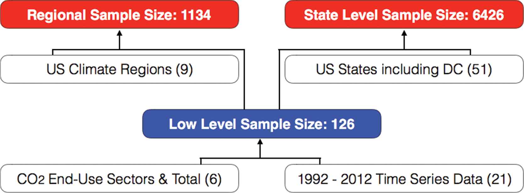
Structure of data with sample size in each level.
Figure 2 shows the data structure based on nine US climate regions with five end-use sectors, and the following data modification enables us to perform a transitional modeling of the data.
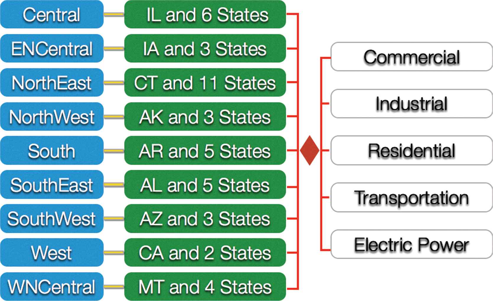
Illustration of US climate regions with CO2 emission sectors.
2.2. Transitional Modeling
The key idea of the present study is predicting the probability that the changing rate of the CO2 emission in a specific region is higher than the average changing rate based on values of attributable variables in the past over all climate regions. While we use the past response values as independent variables in direct transitions for the ordinary transitional modeling [17,18], the indirect transition method has been applied in the present study. In other words, our interest in this modeling procedure is on the statistical modeling of
The Equation (1) below represents the theoretical indirect transition model of the regional data, and Equation (2) shows the fitted probability models for all nine US climate regions along with the table of the estimated coefficients.
| 1 | 2 | 3 | 4 | 5 | 6 | 7 | 8 | 9 | |
|---|---|---|---|---|---|---|---|---|---|
| Region | C | ENC | NE | NW | S | SE | SW | W | WNC |
| Region | |||||||
|---|---|---|---|---|---|---|---|
| C | −0.3848 | 0.0317 | 0.1005 | −0.9000 | 0.6631 | −0.2748 | 0.5202 |
| ENC | −0.3848 | 0.0774 | −0.5266 | −1.8590 | 0.3162 | 1.6961 | −0.5375 |
| NE | −0.3848 | 0.0593 | 0.1332 | −1.2377 | 0.4604 | 1.0280 | 0.0271 |
| NW | −0.3848 | 0.0092 | −0.3751 | −0.3450 | 0.6133 | 0.4202 | −0.4589 |
| S | −0.3848 | 0.0199 | −0.2813 | −0.4035 | 0.9975 | −0.4903 | −0.5316 |
| SE | −0.3848 | 0.0421 | −0.5519 | −0.9326 | 0.2614 | 0.2175 | 0.2121 |
| SW | −0.3848 | −0.0296 | −0.3225 | −0.6208 | 0.3235 | 1.0365 | −0.3863 |
| W | −0.3848 | 0.0361 | −0.5263 | −0.5422 | −0.4334 | 0.5534 | 0.5709 |
| WNC | −0.3848 | −0.0326 | 0.2560 | 1.3760 | −0.2732 | −0.4342 | −0.0973 |
Estimated coefficients in the Equations (2).
Probabilities that the CO2 emission in each region is more than the average US CO2 emission at
| S1 | S2 | S3 | S4 | S5 | C | ENC | NE | NW | S | SE | SW | W | WNC |
|---|---|---|---|---|---|---|---|---|---|---|---|---|---|
| 0 | 0 | 0 | 0 | 0 | 0.5852 | 0.8015 | 0.7269 | 0.4568 | 0.5182 | 0.6419 | 0.2562 | 0.6096 | 0.2433 |
| 1 | 0 | 0 | 0 | 0 | 0.6094 | 0.7045 | 0.7526 | 0.3663 | 0.4481 | 0.5079 | 0.1997 | 0.4798 | 0.2935 |
| 0 | 1 | 0 | 0 | 0 | 0.3645 | 0.3861 | 0.4357 | 0.3733 | 0.4181 | 0.4136 | 0.1562 | 0.4758 | 0.5601 |
| 0 | 0 | 1 | 0 | 0 | 0.7325 | 0.8470 | 0.8084 | 0.6083 | 0.7447 | 0.6995 | 0.3225 | 0.5030 | 0.1966 |
| 0 | 0 | 0 | 1 | 0 | 0.5174 | 0.9565 | 0.8815 | 0.5614 | 0.3971 | 0.6902 | 0.4927 | 0.7308 | 0.1724 |
| 0 | 0 | 0 | 0 | 1 | 0.7036 | 0.7022 | 0.7323 | 0.3470 | 0.3873 | 0.6890 | 0.1897 | 0.7343 | 0.2258 |
| 1 | 1 | 0 | 0 | 0 | 0.3881 | 0.2709 | 0.4687 | 0.2904 | 0.3516 | 0.2888 | 0.1183 | 0.3491 | 0.6218 |
| 1 | 0 | 1 | 0 | 0 | 0.7517 | 0.7658 | 0.8282 | 0.5162 | 0.6876 | 0.5727 | 0.2564 | 0.3742 | 0.2402 |
| 1 | 0 | 0 | 1 | 0 | 0.5424 | 0.9286 | 0.8948 | 0.4680 | 0.3321 | 0.5620 | 0.4130 | 0.6160 | 0.2120 |
| 1 | 0 | 0 | 0 | 1 | 0.7241 | 0.5821 | 0.7576 | 0.2675 | 0.3230 | 0.5606 | 0.1450 | 0.6201 | 0.2737 |
| 0 | 1 | 1 | 0 | 0 | 0.5268 | 0.4632 | 0.5503 | 0.5238 | 0.6608 | 0.4781 | 0.2038 | 0.3705 | 0.4921 |
| 0 | 1 | 0 | 1 | 0 | 0.3035 | 0.7743 | 0.6834 | 0.4755 | 0.3056 | 0.4671 | 0.3430 | 0.6122 | 0.4519 |
| 0 | 1 | 0 | 0 | 1 | 0.4911 | 0.2687 | 0.4424 | 0.2735 | 0.2969 | 0.4658 | 0.1118 | 0.6164 | 0.5360 |
| 0 | 0 | 1 | 1 | 0 | 0.6754 | 0.9679 | 0.9218 | 0.7027 | 0.6411 | 0.7431 | 0.5731 | 0.6377 | 0.1368 |
| 0 | 0 | 1 | 0 | 1 | 0.8217 | 0.7639 | 0.8125 | 0.4953 | 0.6315 | 0.7421 | 0.2445 | 0.6418 | 0.1817 |
| 0 | 0 | 0 | 1 | 1 | 0.6433 | 0.9278 | 0.8843 | 0.4472 | 0.2791 | 0.7336 | 0.3976 | 0.8278 | 0.1589 |
| 1 | 1 | 1 | 0 | 0 | 0.5518 | 0.3376 | 0.5830 | 0.4305 | 0.5952 | 0.3453 | 0.1564 | 0.2580 | 0.5558 |
| 1 | 1 | 0 | 1 | 0 | 0.3252 | 0.6695 | 0.7115 | 0.3839 | 0.2493 | 0.3355 | 0.2744 | 0.4826 | 0.5158 |
| 1 | 1 | 0 | 0 | 1 | 0.5162 | 0.1783 | 0.4754 | 0.2055 | 0.2417 | 0.3343 | 0.0835 | 0.4870 | 0.5987 |
| 1 | 0 | 1 | 1 | 0 | 0.6970 | 0.9469 | 0.9309 | 0.6190 | 0.5741 | 0.6249 | 0.4930 | 0.5098 | 0.1699 |
| 1 | 0 | 1 | 0 | 1 | 0.8359 | 0.6564 | 0.8320 | 0.4028 | 0.5640 | 0.6237 | 0.1899 | 0.5142 | 0.2229 |
| 1 | 0 | 0 | 1 | 1 | 0.6660 | 0.8836 | 0.8973 | 0.3573 | 0.2261 | 0.6133 | 0.3235 | 0.7395 | 0.1962 |
| 0 | 1 | 1 | 1 | 0 | 0.4582 | 0.8247 | 0.7738 | 0.6260 | 0.5440 | 0.5324 | 0.4191 | 0.5058 | 0.3856 |
| 0 | 1 | 1 | 0 | 1 | 0.6519 | 0.3352 | 0.5570 | 0.4100 | 0.5338 | 0.5311 | 0.1481 | 0.5102 | 0.4678 |
| 0 | 1 | 0 | 1 | 1 | 0.4230 | 0.6671 | 0.6892 | 0.3643 | 0.2055 | 0.5201 | 0.2619 | 0.7365 | 0.4280 |
| 0 | 0 | 1 | 1 | 1 | 0.7778 | 0.9464 | 0.9238 | 0.5990 | 0.5121 | 0.7815 | 0.4770 | 0.7570 | 0.1257 |
| 1 | 1 | 1 | 1 | 0 | 0.4833 | 0.7354 | 0.7962 | 0.5350 | 0.4738 | 0.3960 | 0.3432 | 0.3768 | 0.4477 |
| 1 | 1 | 1 | 0 | 1 | 0.6744 | 0.2294 | 0.5895 | 0.3232 | 0.4636 | 0.3947 | 0.1119 | 0.3810 | 0.5317 |
| 1 | 1 | 0 | 1 | 1 | 0.4477 | 0.5420 | 0.7170 | 0.2825 | 0.1633 | 0.3843 | 0.2045 | 0.6228 | 0.4915 |
| 1 | 0 | 1 | 1 | 1 | 0.7947 | 0.9124 | 0.9326 | 0.5066 | 0.4421 | 0.6732 | 0.3979 | 0.6480 | 0.1567 |
| 0 | 1 | 1 | 1 | 1 | 0.5873 | 0.7333 | 0.7785 | 0.5141 | 0.4122 | 0.5847 | 0.3290 | 0.6443 | 0.3628 |
| 1 | 1 | 1 | 1 | 1 | 0.6114 | 0.6188 | 0.8006 | 0.4210 | 0.3461 | 0.4477 | 0.2621 | 0.5170 | 0.4238 |
Probabilities for all possible cases.
3. CLUSTER ANALYSIS
We develop six cluster maps showing the atmospheric CO2 emission regions in the United States based on effects of the total CO2 emission and all five end-use sectors; the commercial, electric power, industrial, residential, and transportation sector. After normalizing the probability data in Table 1 using Johnson's transformation [19] and [20], the hierarchical clustering procedure has been performed using Ward's method, in which we consider a clustering problem as a problem of minimizing within-cluster sum of squares in each cluster rather than a distance problem [21–23]. In Ward's method, we begin with nine clusters of size 1 and combine two clusters that render the minimum error sum of squares in Equation (3), or yield maximum
Table 2 illustrates the results of the hierarchical clustering using Ward's method based on effects of total CO2 emission, the commercial, electric power, industrial, residential, and transportation sector denoted by Total,
| Region | Clustering Based on |
|||||
|---|---|---|---|---|---|---|
| Total | ||||||
| C | C 1 | C 1 | C 2 | C 2 | C 2 | C 2 |
| ENC | C 2 | C 2 | C 2 | C 1 | C 3 | C 3 |
| NE | C 2 | C 1 | C 2 | C 1 | C 1 | C 1 |
| NW | C 1 | C 2 | C 1 | C 2 | C 1 | C 3 |
| S | C 1 | C 2 | C 1 | C 2 | C 2 | C 3 |
| SE | C 1 | C 3 | C 2 | C 1 | C 1 | C 1 |
| SW | C 3 | C 2 | C 1 | C 1 | C 3 | C 3 |
| W | C 1 | C 3 | C 1 | C 3 | C 1 | C 2 |
| WNC | C 3 | C 1 | C 3 | C 3 | C 2 | C 1 |
| 0.566 | 0.869 | 0.838 | 0.898 | 0.853 | 0.822 | |
Clustering based on different factors.
3.1. Clustering Based on the Effect of the Total CO2 Emissions
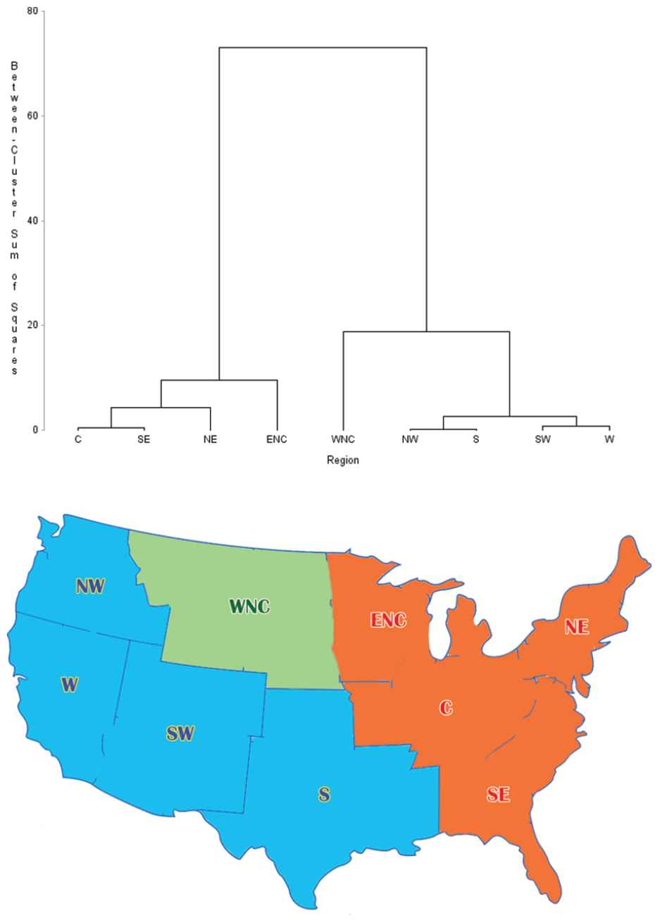
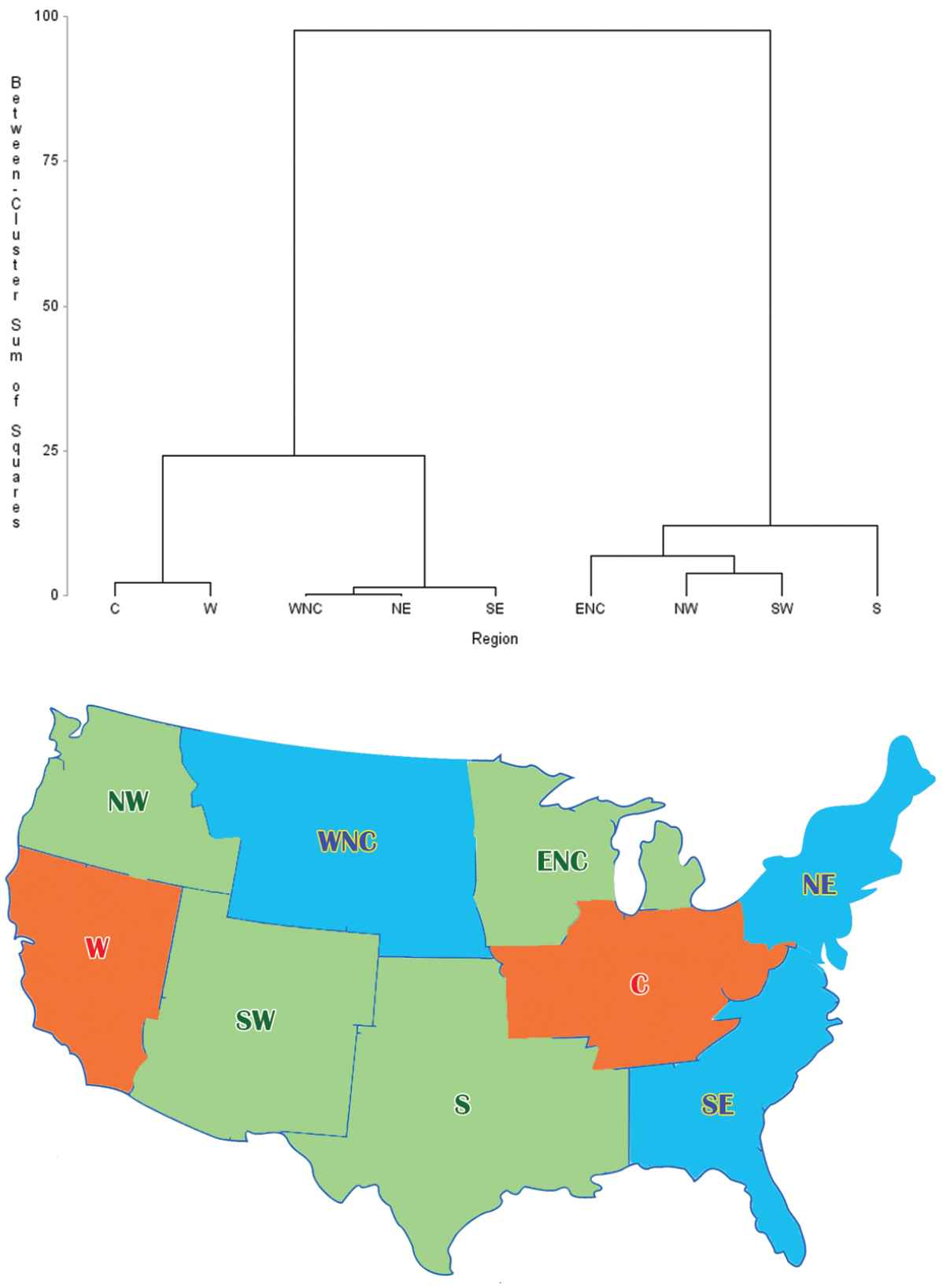
In Figure 3, we see that nine US climate regions are combined into three CO2 emission clusters based on the effect of the total CO2 emission.
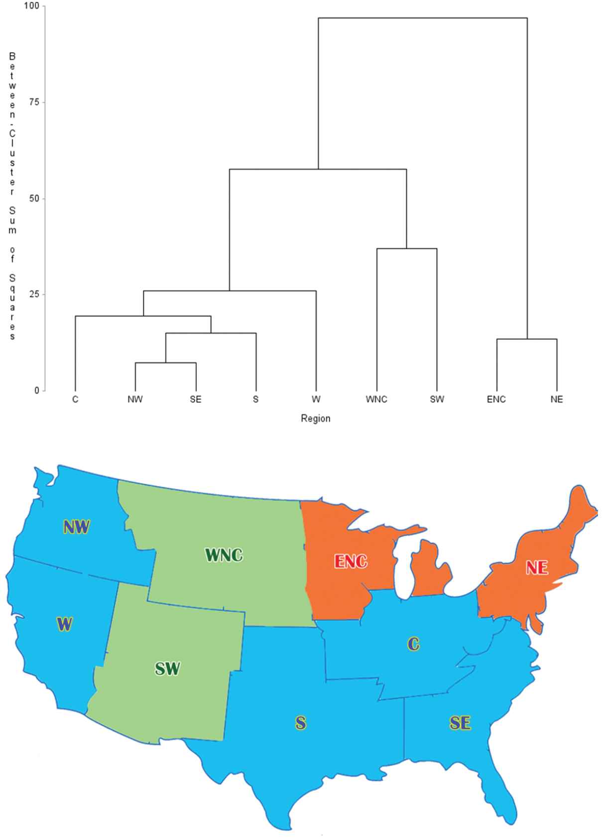
Dendrogram and cluster map based on the effect of the total CO2 emission.
The cluster 1 consists of five US climate regions; the central, northwest, south, southeast, and west regions, and the cluster 2 is composed of the east north central and northeast regions. Finally the remaining two regions; the west north central and southwest regions, build the cluster 3. Regions in the same cluster share common characteristics with respect to the clustering criterion, and the total CO2 emission criterion yields geographical clustering results and this tells that the total CO2 emission is highly related to the geographic climate condition.
3.2. Clustering Based on the Effect of the Commercial Sector
The commercial sector includes all businesses except manufacturing and transportation, and any CO2 emissions from related fossil fuels combustion such as heating, driving, and other activities within business purposes are counted to the commercial CO2 emissions.
Figure 4 displays three-cluster solution by the commercial sector criterion. The west region and the southeast region have similar characteristics with respect to the commercial aspect and this seems to be proved by The Walt Disney Company because two Disney resorts, Disney World and Disney Land, are located in these two regions. The other two clusters are also comprised of regions with similarity upon the commercial sector criterion.
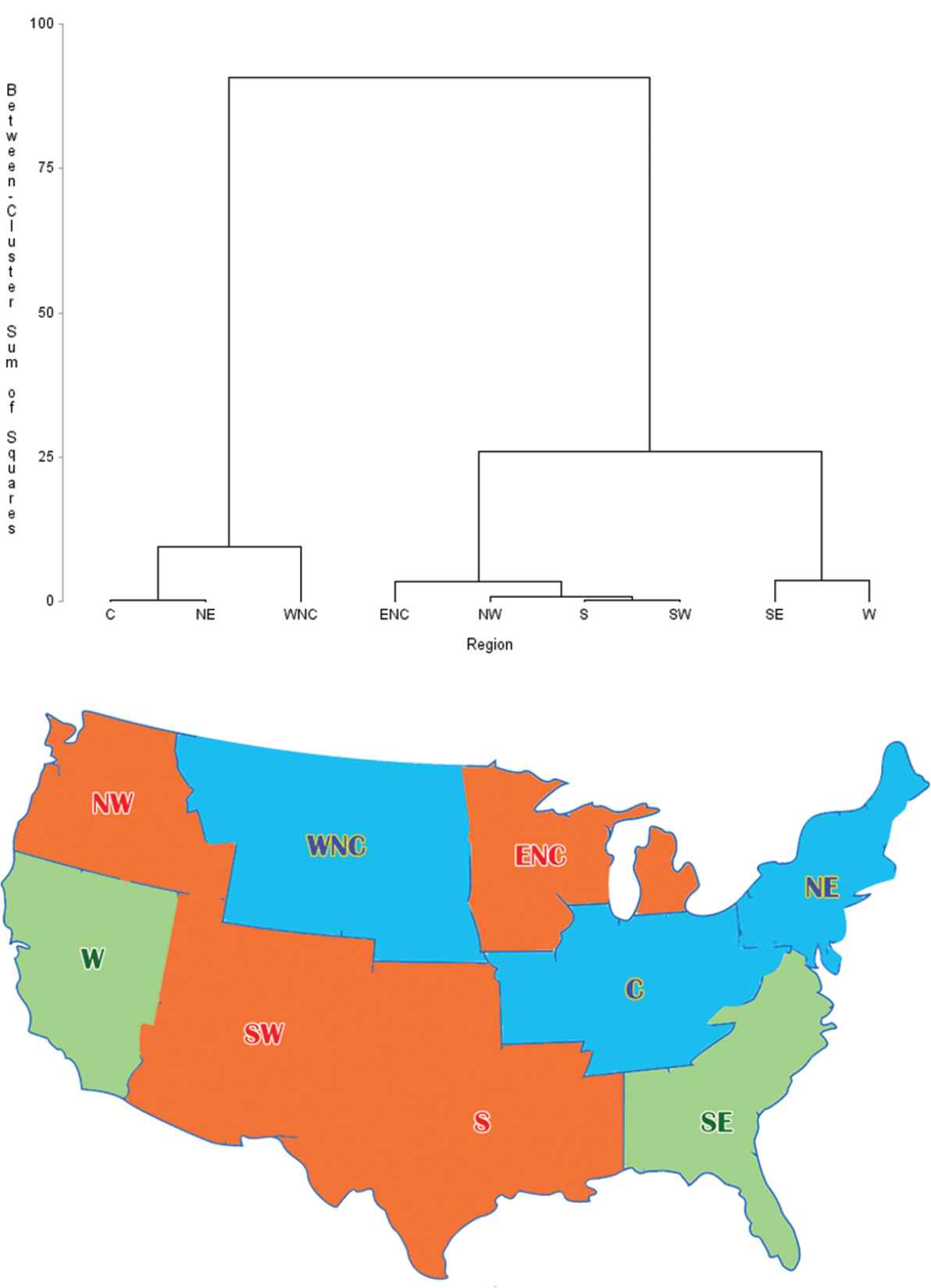
Dendrogram and cluster map based on the effect of the commercial sector.
3.3. Clustering Based on the Effect of the Electric Power Sector
The electric power sector not only involves the generation of the electricity but also includes transmission and distribution of the electricity. The CO2 emission from the electric power sector makes up about 32% of the total amount of CO2 emission in the United States and this is the top contributing sector among all five sectors to the CO2 emission in the United States.
The electric power sector criterion also highlights three-cluster solution with reasonably well combined cluster map in Figure 5. The relationship between the electric power sector and the CO2 emission can be found in the source of the electric power and the amount of the electric usage. The geographical distribution of the type of the major power plants in Figure 6 proves such a relationship. Most of the steam and nuclear power plants are located in the cluster with the southeast, central, east north central, and northeast regions, whereas we find major hydroelectric power plants in the cluster with the northwest, west, southwest, and south regions.
Dendrogram and cluster map based on the effect of the electric power sector.
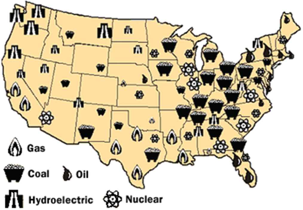
A breakdown of the major power plants in the United States, by type.
3.4. Clustering Based on the Effect of the Industrial Sector
The industrial sector emits the CO2 directly and indirectly to our atmosphere. The direct way of emissions involves burning fossil fuels to produce commercial goods, and the CO2 emission at a power plant to generate electricity to use in industrial facilities is categorized to the indirect way of emissions. The industrial sector occupies around 20% of total CO2 emissions in the United States.
Figure 7 shows similarities between the west and west north central regions, among the northwest, south, and central regions, and among the other four regions. In order to control the CO2 emission from the industrial aspect in each cluster, we need further scientific research, which may suggest re-location of chemical plants that may have significant interaction effects, as a solution of reducing CO2 emission nationwide.
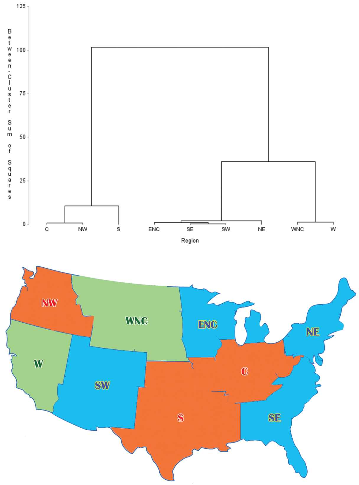
Dendrogram and cluster map based on the effect of the industrial sector.
3.5. Clustering Based on the Effect of the Residential Sector
The residential sector increases the atmospheric CO2 concentration through heating, cooking, and other home maintaining activities. Although the contribution of the residential sector to the total CO2 emission is less than 10% in the United States, it is very important to control the emission due to the residential sector because every individual is a member of this residential sector and the effect of a campaign against the CO2 emission may reach all other sectors.
Clustering based on the residential sector criterion also provides three-cluster solution in Figure 8. One remarkable feature of this clustering is that the cluster, comprised of the northwest, west, northeast, and southeast regions, includes all the Pacific and Atlantic seaside regions, while other inland regions form the other two clusters. It is very interesting that the effect of the residential aspect to the CO2 emission is related to the human lifestyle founded on the geographic characteristics.
Dendrogram and cluster map based on the effect of the residential sector.
3.6. Clustering Based on the Effect of the Transportation Sector
The transportation sector produces the atmospheric CO2 through the movement of merchandise and people by the combustion of petroleum-based products such as gasoline, diesel, and bunker fuels. This sector has the second greatest contribution to the total CO2 emissions, about 28%, in the United States.
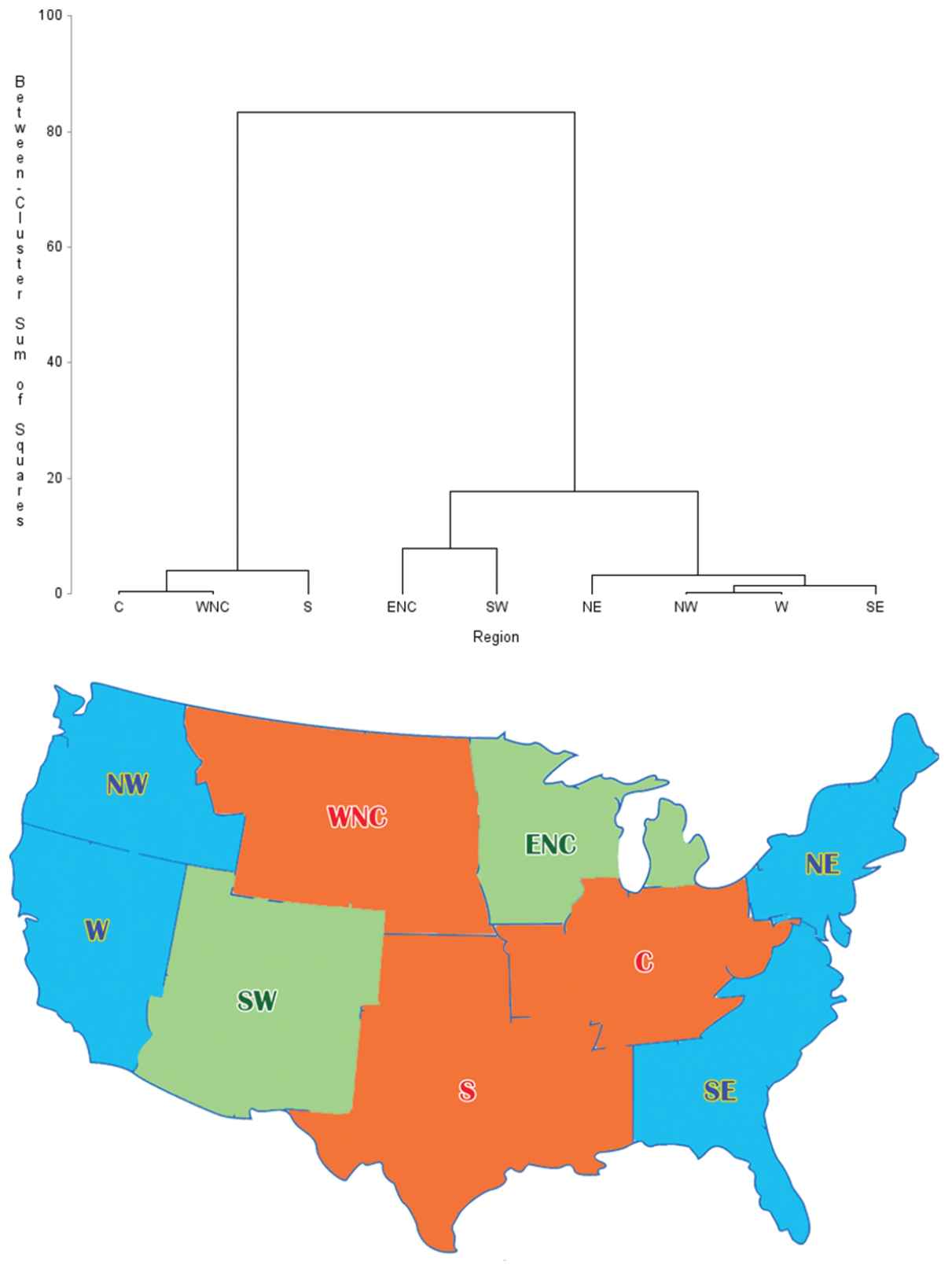
Figure 9 shows similarities between the west and central regions, among the southeast, northeast, and west north central regions, and all remaining regions. This three-cluster solution provides reasonable evidence to share regulations to reduce the CO2 emission in a transportation aspect for regions within the same cluster.
Dendrogram and Cluster Map based on the Effect of the Transportation Sector.
4. CONCLUSION
The present study provides several guidelines, for policy makers, to effectively control the level of the carbon dioxide emissions in each US climate region. Firstly, fitted regional probability models driven by Equation (2), derived from transitional models in Equation (1), that allow us to calculate the probabilities of the CO2 emission at risk in each region based on all possible combinations of by-sector CO2 emission behaviors in the previous year. Ranks of the effect of by-sector behaviors to the level of the CO2 emissions in each climate region are displayed in Table 3, below.
| Region | Ranks with Maximum Probability |
|||
|---|---|---|---|---|
| Rank 1 | Rank 2 | Rank 3 | Max. Prob. | |
| C | S3 | S5 | S1 | 0.8359 |
| ENC | S4 | S3 | S1 | 0.9679 |
| NE | S4 | S3 | S1 | 0.9326 |
| NW | S3 | S4 | S2 | 0.7027 |
| S | S3 | S1 | S2 | 0.7447 |
| SE | S3 | S4 | S5 | 0.7815 |
| SW | S4 | S3 | S1 | 0.5731 |
| W | S5 | S4 | S3 | 0.8278 |
| WNC | S2 | S1 | S5 | 0.6218 |
Ranks of sectors with maximum probabilities in each region.
We can conclude that the number one risk sector in the central region is S3, the industrial sector, the number two risk sector is S5, the transportation sector, and the rank three sector is S1, the commercial sector. Accordingly, the industrial sector CO2 emission has a role of a preceding index when we predict how the CO2 emission changes in the following year for the central region. Similarly, we consider the residential sector CO2 emission as a preceding index for the east north central region, the transportation sector CO2 emission as a leading index for the west region, and so on. Moreover, ranks in Table 3 are assigned under consideration of interaction effects among all possible combinations of five sectors. Secondly, we can effectively control the total CO2 emission using CO2 clusters by the effect of each sector shown in Table 2. For instance, we may apply the same policy regarding the residential sector to all west and east coastal regions because they share similar properties within residential related problems as shown in Figure 8.
Providing a solution to an environmental problem is not so simple because most environmental problems are due to human activities that are not predictable. However, these statistical models would be a strong background for our government to legislate more effective regulations to control the optimal level of the CO2 emission in the United States on regional basis.
ACKNOWLEDGEMENTS
The authors would like to acknowledge many fruitful discussions with Ram C. Kafle at Sam Houston State University and Bhikhari Tharu at Spelman College.
REFERENCES
Cite this article
TY  - JOUR
AU  - Doo Young Kim
AU  - Chris P. Tsokos
PY  - 2020
DA  - 2020/03/03
TI  - A Stochastic Approach in Modeling of Regional Atmospheric CO2 in the United States
JO  - Journal of Statistical Theory and Applications
SP  - 10
EP  - 20
VL  - 19
IS  - 1
SN  - 2214-1766
UR  - https://doi.org/10.2991/jsta.d.200224.002
DO  - 10.2991/jsta.d.200224.002
ID  - Kim2020
ER  -