Journal of Statistical Theory and Applications

Volume 18, Issue 4, December 2019, Pages 439 - 449

A New F-Test Applicable to Large-Scale Data

Authors
Mohsen Salehi1, 2, Adel Mohammadpour2, *, Kerrie Mengersen3
1Department of Statistics, University of Qom, Qom, Iran
2Department of Statistics, Amirkabir University of Technology (Tehran Polytechnic), Tehran, Iran
3Science and Engineering Faculty, Queensland University of Technology, Brisbane, Australia
*Corresponding author. Email: adel@aut.ac.ir
Corresponding Author
Adel Mohammadpour
Received 25 May 2017, Accepted 6 June 2018, Available Online 27 December 2019.
DOI
10.2991/jsta.d.191217.001How to use a DOI?
Keywords
Microarray data; Permutation test; Null statistic; F-test
Abstract

In large-scale multiple testing, the permutation test based on making a null statistic has been widely employed in the literature. Because it enables us to use the null permuted samples and estimate the p-value more accurately. Some test statistics, which can be modified to a null statistic, have been proposed for two independent groups. In this paper, we propose a new statistic and corresponding F-test, which can be applied for three or more groups. The simulation results demonstrate that the proposed method has a smaller interquartile range (IQR) than the usual permutation method and estimates p-values more accurately than its rival.

Copyright
© 2019 The Authors. Published by Atlantis Press SARL.
Open Access
This is an open access article distributed under the CC BY-NC 4.0 license (http://creativecommons.org/licenses/by-nc/4.0/).

1. INTRODUCTION

In some experimental scientific fields such as microarray and deep sequencing (or next generation sequencing) methods in biology, the numbers of features (probe sets) is huge while the number of samples is limited to perhaps only two or three. Nearly all features are numeric, showing the values of gene expressions between control and other groups, and finding differentially expressed genes between those groups is of great interest. Such data refer to large-scale data.

Traditional approaches to multiple testing under a null hypothesis, the equality of means in different groups, can lead to inaccurate decisions, particularly in the context of many tests and small sample sizes. These poor decisions can arise for a number of reasons, including the detection of spurious significant differences, asymmetry in the distribution of alternatives [1], and failure of assumptions about the normality of the underlying random variables. In this situation, employing the permutation method to estimate the p-values using the permutation samples has been recommended [211]. In addition, in some multiple hypothesis testing, the distribution of alternatives is not symmetric, and we need some alternative methods in this situation, see [1].

However, as the sample size is small, the number of permutation samples is reduced and the estimation of an appropriate p-value seems unreachable. In addition, using the permutation samples, the samples in two types of groups, which are measured under two conditions (i.e., time point), are being mixed together. Then, multiple testing under the null hypothesis is done, which we know that the null hypothesis is not satisfied for many of them. In fact, the permuted samples may not permit resampling from the null distribution of the test statistic, which is called the null permuted sample. Therefore, the usual permutation method cannot be used to estimate the p-value directly.

To overcome this obstacle one can use the null statistic. The null statistic is a modified test statistic from the initial test statistic with the same distribution. Some methods based on deriving a null statistic have been constructed for the analysis of two groups, e.g., see [4,12]. However, in many cases, interest may center on three or more groups. For instance, in microarray analysis introduced by [1315], three groups were used to describe the expression value of many genes.

Some researchers have proposed three-stage filtrations, which reduce the number of comparisons and then use one-way analysis of variance (ANOVA) to identify the differentially expressed genes on filtered genes or features, see [13], and also [16,17]. Applying one-way ANOVA and calculating the p-values and subjecting them to a new approach, namely a Beta Contamination model, has also been reported; see [16]. In brief, in [13,16] the p-values estimated by a traditional F-test are used as the starting point of a subsequent statistical analysis, whereas in [17] ANOVA is employed to identify differentially expressed genes from next generation sequencing and microarray in transcriptome profiling of activated T cells. In addition, some widely used tools in these fields like RMAexpress, which compute the summary of values of gene expression, using the obtained p-values from ANOVA for screening huge numbers of differentially expressed genes, see [1820]. This literature motivates the development of a new test statistic to facilitate estimation of more accurate p-values in multiple hypothesis testing with three or more groups.

We organize the paper as follows: In Section 2, we review the Fisher test, the usual permutation test for the one-way ANOVA, and the estimation of the p-value using the null statistic. We propose a new test statistic, which is modified to a null statistic in Section 3. To investigate the robustness of the proposed test statistic and accuracy of the estimated p-values, some simulation studies are presented in Section 4. In this section, two real data sets are also considered. Finally, the conclusions are given in Section 5.

2. F-TEST AND PERMUTATION SOLUTION

When we have three independent groups or more and we are going to test the null hypothesis, equality of means, versus the alternative hypothesis, different means, we usually use the well-known one-way ANOVA method, under the assumption of normally distributed, independent random samples in each group. When the normality assumption is not satisfied, we can use the permutation method instead. In this section, we review these methods briefly. In addition, we present a method for estimating the p-value based on the permutation method in large-scale data.

2.1. Multiple Testing Problems

In this paper, we deal with multiple hypothesis testing with k independent groups. For ease of exposition, we consider a single test. Let X1,X2,,Xk be the underlying random variables in k groups, and μ1,μ2,,μk be the corresponding means, respectively with common variance σ2. Let Xi=Xi1,Xi2,,Xini, i=1,2,,k is the vector of random samples from Xi's. Take Z=X1,X2,,Xk. We are going to test the following hypotheses:

{H0:μ1=μ2==μkH1:μiμj,ij.(1)

A common test statistic, which is used for testing the hypotheses (1) is the Fisher test, [21], as follows:

FZ=i=1kniX¯i.X¯2k1i=1kj=1niXijX¯i.2Nk,(2)
where
X¯i.=j=1niXijni,X¯=i=1kj=1niXijN,
and N=i=1kni. If we consider the normality assumption for the underlying variables in each group, the distribution of F in (2), under the null hypothesis will be F distribution with k1 and Nk degrees of freedom.

In the usual permutation approach described by [22], one constructs (2) by randomly permuting

Z=X1,X2,,Xk=X11,,X1n1,X21,,X2n2,,Xk1,,Xknk.

Denote the permuted elements of Z by Z and let Xij denote the jth permutation sample in the ith group. Then, X1 and Xk are the first n1 and the last nk random samples of Z. Clearly, the F statistic with permutation samples denoted as F=FZ, has also the F distribution.

2.2. Estimated p-Value

Suppose that we decide to reject the null hypothesis H0 when the test statistic FZ is sufficiently large. Therefore, the p-value can be defined by

p=PrFZf|H0,
where f is the observed value of FZ. If we consider the B permutation samples and denote Zb as a bth permutation sample of Z, then the estimator of the p-value can be defined as follows:
p̂=1Bb=1BIFZbf,(3)
where ID denotes the indicator function: ID is one if D is satisfied, and is zero if is not.

In large-scale data like microarray data, we can use the information of other genes to estimate the p-value for a special gene with higher accuracy. A good alternative for the p-value estimator is defined by

p̂FZ;fg=1BGb=1Bg=1GIFZbtfg,(4)
where Zbt and fg are the bth permutation sample at the tth gene and the observed value of the test statistic of the gth gene, respectively.

(3) and (4) involve the use of information about a lot of genes, and it is unknown if the null hypothesis holds for them. [11] and [4] suggest the usage of the null statistic instead of the main test statistic. The null statistic, FnullZ, is a test statistic with the same distribution as the initial test statistic, FZ, such that

pFZ;f=PrFZf|H0=PrFnullZf.(5)

Therefore, one can estimate the p-value more accurately as follows:

p̂FnullZ;fg=1BGb=1Bg=1GIFnullZbtfg.(6)

3. PROPOSED METHOD

We propose a new permutation test statistic for hypothesis testing (1), such that it can be modified to a null statistic. The p-values are estimated by (6).

Constructing the test statistic and its null statistic: Consider Xi=Xi1,Xi2,,Xini for i=1,2,,k. We divide the sample size of the ith group into two partitions, with ni1 and ni2 elements,

Xi(1)=Xi1,Xi2,,Xini1,Xi(2)=Xini1+1,Xini1+2,,Xini,(7)
such that, ni=ni1+ni2. Take
X¯i(1)=j=1ni1Xijni1,X¯i(2)=j=ni1+1niXijni2.

We want to test the hypotheses (1).

Theorem 3.1.

Under the normality assumption for Xi, where i=1,2,,k, and under the null hypothesis, the test statistic for testing (1) given by

FsZ=i=1kniX¯i(1)+X¯i(2)i=1kniX¯i(1)+X¯i(2)i=1kni2k1i=1kl=12nil1Sil2N2k,(8)
where
1ni=1ni1+1ni2,Sil2=1nil1j=1nilXijX¯il2
has an F distribution with k1 and N2k degrees of freedom, respectively.

Proof.

Let k=2, U¯1=X¯1(1)+X¯1(2) and U¯2=X¯2(1)+X¯2(2). Assuming a normal distribution for X1 and X2, the distribution of U¯1U¯2 is given by

U¯1U¯2N2μ12μ2,1n11+1n12+1n21+1n22σ2.

Since Xi, i=1,2, are independent, then Xi(1), Xi(2) are also independent. On the other hand, if we define Si2 as the variance of the random sample in the ith group, we know that (ni1)Si2σ2 has a Chi-squared distribution with (ni1) degrees of freedom. Then, nil1Sil2σ2, for i=1,2, and l=1,2, are also independent and have a Chi-square distribution with the nil1 degrees of freedom. Let S2=i=12l=12nil1Sil2, then N4S2σ2 has a Chi-squared distribution with N4 degrees of freedom. Thus, the distribution of U¯1U¯2σ1n1+1n2 is the standard normal distribution under the null hypothesis μ1=μ2. We can rewrite U¯1U¯21n1+1n2 as follows:

U¯1U¯21n1+1n22=U¯1U¯2Nn1n22,=n2n1NU¯1U¯22+n1n2NU¯1U¯22,=n2U¯2+n1U¯1+n2U¯2N2+n1U¯1n1U¯1+n2U¯2N2,
where N=n1+n2. Suppose that U¯¯=n1U¯1+n2U¯2N, then
U¯1U¯21n1+1n22=i=12niU¯iU¯¯2.(9)

It can be shown that U¯1U¯2 and S2 are independent [4], so (9) is independent of S2. Thus, U¯1U¯2S1n1+1n2 has a t-distribution with N4 degrees of freedom. Therefore,

i=12ni(U¯iU¯¯)2S2/N4,
has a Fisher distribution with 21 and N2×2 degrees of freedom. In fact, U¯i and U¯¯ are the weighted means of the ith group and total sample, respectively. Therefore,
FsZ=i=1kniX¯i(1)+X¯i(2)i=1kniX¯i(1)+X¯i(2)i=1kni2k1i=1kl=12nil1Sil2N2k,
has a Fisher distribution with k1 and N2k degrees of freedom.

Remark 3.1.

It follows, from Theorem 3.1, that for testing the null hypothesis in (1), the test statistic Fm is of level α. The corresponding null statistic is given by

FsnullZ=i=1kniX¯i(1)X¯i(2)i=1kniX¯i(1)X¯i(2)i=1kni2k1i=1kl=12nil1Sil2N2k.(10)

The critical value, called c, is determined such that PrFsZc|H0=α.

Theorem 3.2.

Fs and Fsnull statistics satisfy the following condition:

PFsZ>fs|H0=PFsnullZ>fs,fsIR.

Proof.

Since the denominator of FsZ and FsnullZ is the same, it is enough to show that the distribution of T1=X¯i(1)+X¯i(2)i=1kniX¯i(1)+X¯i(2)i=1kni under the null hypothesis is the same as for distribution of T2=X¯i(1)X¯i(2)i=1kniX¯i(1)X¯i(2)i=1kni. It is evident that the distributions of X¯i(1)+X¯i(2) and i=1kniX¯i(1)+X¯i(2)i=1kni follow normal distributions with means 2μi, 2i=1kniμiN and variances σ2ni and σ2j=1kni, respectively. Therefore, under the null hypothesis, T1 follows a zero-mean normal distribution with variance σ21ni+1i=1kni. Similarly, X¯i(1)X¯i(2) and i=1kniX¯i(1)X¯i(2)i=1kni have zero-mean normal distributions with variances σ2ni and σ2j=1kni, respectively. This implies that both T1 and T2 have the same distribution.

Remark 3.2.

To estimate the p-value in each test, each group is divided into two partitions as (9) and computed the observed value of (8), fs. Then, the samples in all groups are permuted in all tests separately and randomly; and computed (10) for all of them. The p-value can be estimated by (6).

4. RESULTS

This section is organized into two parts. In the first subsection, the robustness of the proposed test statistic, FsZ and accuracy of the estimated p-value are inspected through some simulation studies. In the second subsection, we apply the proposed method and the usual permutation method to two real data sets.

4.1. Simulated Data

Robustness of the new test statistic: The condition (5) is convinced under the normality condition by Theorem 3.2. Considering some candidates for the underlying distribution of the random sample, we investigate if the proposed test statistic, FsZ and the corresponding null statistic, FsnullZ are robust with respect to the departure from normality. In fact, the condition (5) is examined under the violation of the normality assumption.

Without loss of generality, take k=3 and assume three candidates for the underlying distribution: t-Student, Laplace, and Logistic. Two cases are considered for the sample size for each group, n1,n2,n3=4,4,4 and 30,30,30. We then generate the random samples from the candidate distributions and obtain the observed values of FsZ and FsnullZ for their corresponding parameters. The number of iterations is taken to be 10000. The outcomes are analyzed using the Anderson—Darling (AD) test. Table 1 presents the results. For the first candidate, we suppose that the distribution of the random variables in each group is t-Student with the different degrees of freedoms, 4,10,15,25. The obtained p-values indicate that both in small and large sample size, the condition (5) is satisfied. For the second candidate, it is assumed that the underlying variables follow a Logistic distribution. The location and scale parameters are taken to be as μ=0 and σ=1, respectively. Since the proposed test statistic is invariant in location, we only consider μ=0. The obtained p-value verifies that the condition (5) is met. The same conclusion is drawn for the final candidate with the Laplace distribution for the underlying variables.

Sample Sizes
Candidate Distribution Family Parameter n1,n2,n3=4,4,4 n1,n2,n3=30,30,30
tν 4 0.723 0.952
10 0.281 0.569
15 0.992 0.872
25 0.792 0.958
Logistic μ,σ 0,1 0.204 0.569
Laplace μ,σ 0,1 0.339 0.640

AD, Anderson–Darling; The null hypothesis is that two samples come from the common distribution.

Table 1

The estimated p-value by AD-test.

P-value behavior: Since we want to implement the multiple testing, the random samples in each group are simulated for 1000 tests in two categories. In the first category, 90 percent of them are simulated under the null hypothesis, and in the second category, the remaining 10 percent are simulated under the alternative hypothesis. For this purpose, the random samples are generated from N0,1 in the first category, and generated from Nμ1,1, Nμ2,1 and Nμ3,1 in the second category, such that μi,i=1,2,3 are generated from a normal distribution with zero-mean and variance 4, respectively. In each category, we consider three sample sizes: n1,n2,n3=6,6,6,8,8,8, and 10,10,10.

Let fs and f be the observed values of FsnullZ and FZ, respectively when we permute Z. We draw 1000, 2000, 4000 permuted samples from Z=X1,X2,X3 for the different sample sizes n1,n2,n3=6,6,6,8,8,8, and 10,10,10, respectively. Then; we compute fs and f for all permuted samples. In the Usual Permutation Method, called UPM, the p-values are computed through the method described by [22]. In the Proposed Permutation Method, called PPM, they are computed through p̂FsnullZ;fα.

Remark 4.1.

When we consider no effect in the groups, the labels assigned subject to the groups are interchangeable. Therefore, for each permuted sample, the homogeneity of variance must be tested.

Considering the above remark, when we permute a sample, randomly, and divide it into two partitions, some of the obtained permutation samples will display substantive heterogeneity of variances. These so-called extraneous permutation samples (EPSs) should be removed before computing p-values. Figure 1 shows a rate of about 4 to 10 percent of EPS in 1000 comparisons under different values of α and n1,n2,n3. We investigate three cases for the nominal value α=0.05,0.1,0.2. Figure 2 depicts boxplots of the estimated p-values. In each subfigure, the left and right boxplots present the distribution of the estimated p-values in PPM and UPM, respectively.

Figure 1

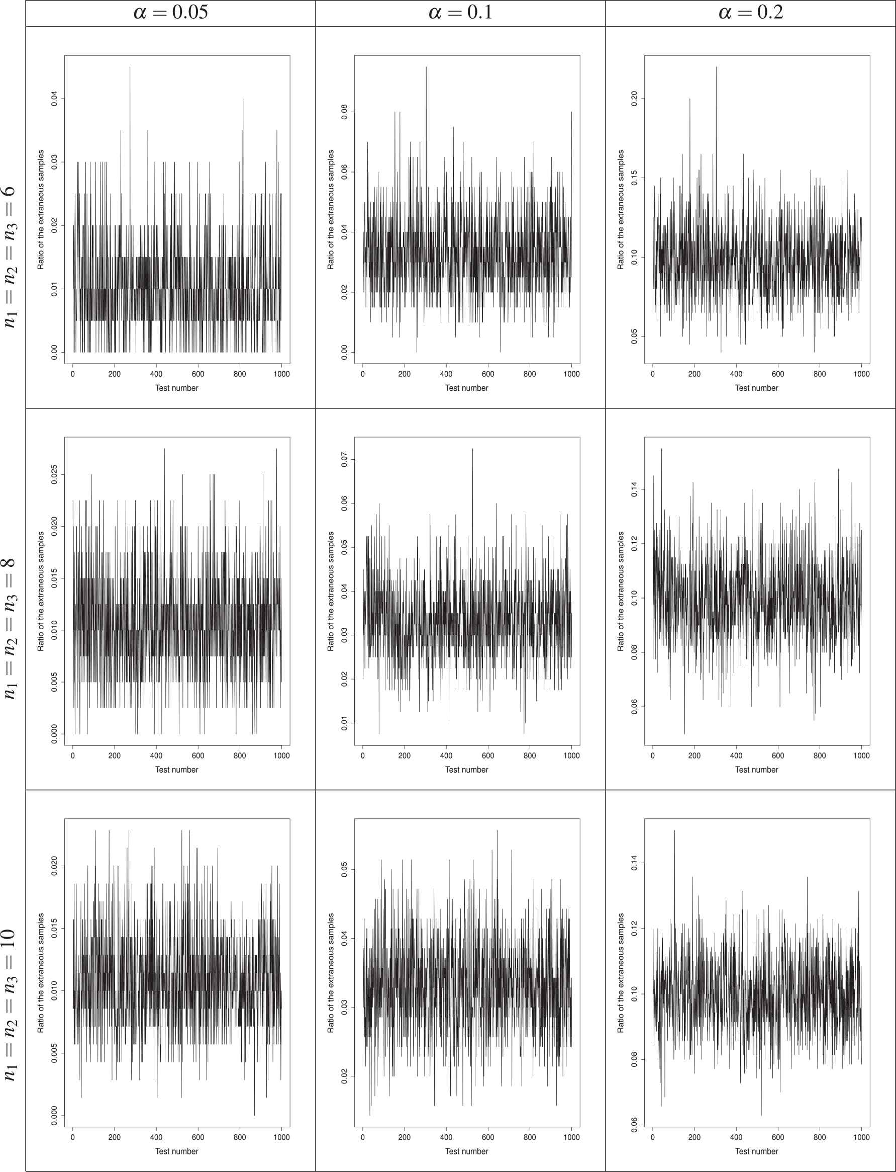
The ratio of extraneous permutation sample (EPS) from the total number of permuted samples in 1000 multiple testing. Each subfigure shows this ratio for the different values of and the sample sizes.

Figure 2

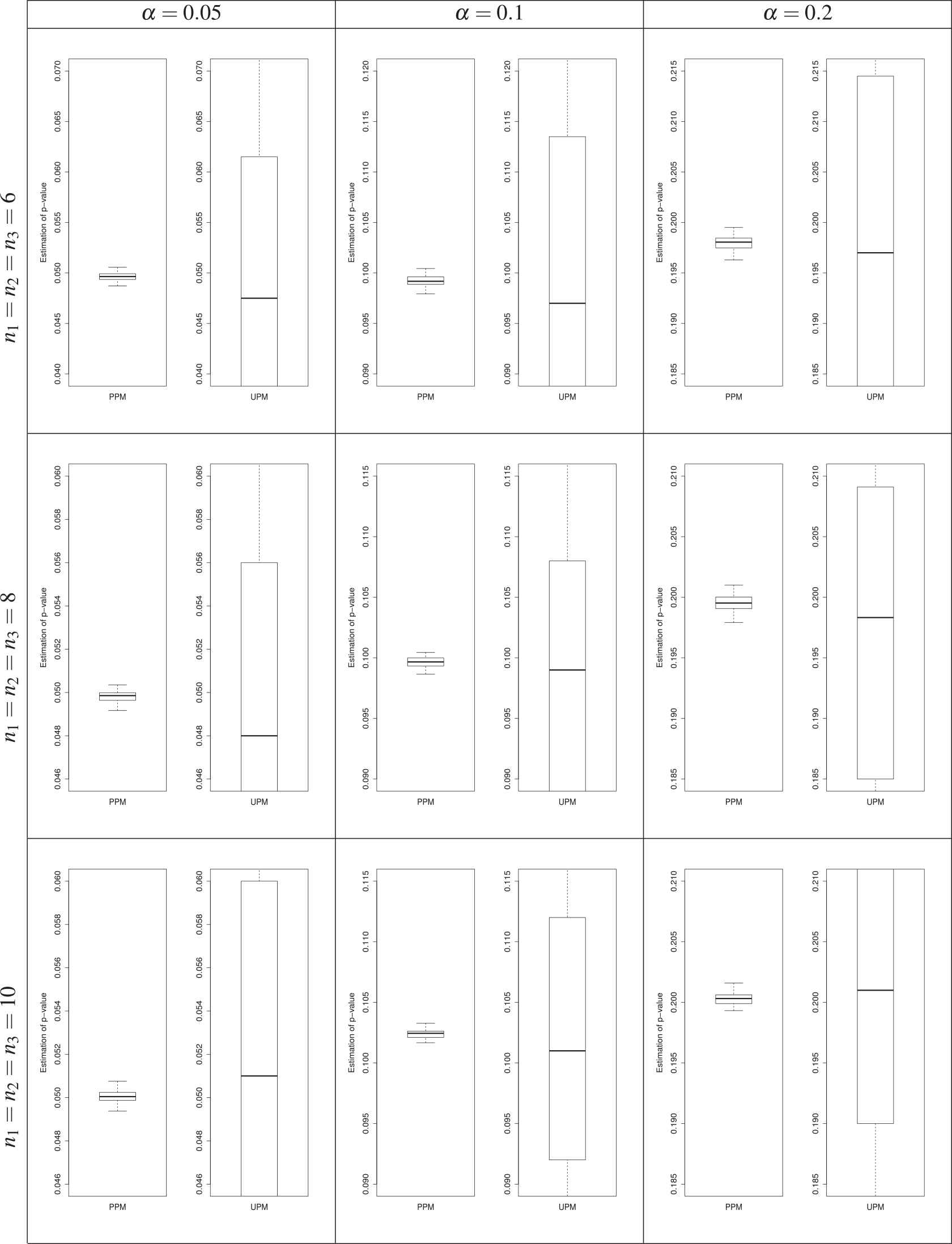
Boxplots of the estimated p-values by UPM and PPM in three cases (n1; n2; n3): (6,6,6), (8,8,8), (10,10,10). The random samples are generated from a normal distribution. UPM and PPM in each sub gure correspond to the usual permutation method and p^(Fsnull(Z);fα)

We can see that the median of the estimated p-values through PPM is closer to the nominal significance levels α than UPM. Moreover, Figure 2 clearly shows that UPM has a considerably higher dispersion than PPM. For more clarity, Table 2 shows the computed interquartile range (IQR) for each subfigure of Figure 1. We can see that the computed IQR for PPM, both with EPS and without EPS, is smaller than for UPM. This simulation study also considered the case in which the distribution is skew-normal with the location, scale, and shape parameters zero, one, and two, respectively. The results are depicted in Figure 3 in this situation.

Sample Sizes n1,n2,n3
(6,6,6)
(8,8,8)
(10,10,10)
α
α
α
Method 0.05 0.1 0.2 0.05 0.1 0.2 0.05 0.1 0.2
UPM 0.0420 0.063 0.0917 0.0350 0.0535 0.0730 0.0302 0.0490 0.0700
PPM with EPS 0.0006 0.0007 0.0011 0.0003 0.0010 0.0007 0.0004 0.0005 0.0005
PPM without EPS 0.0005 0.0007 0.0009 0.0003 0.0006 0.0009 0.0003 0.0005 0.0007

IQR, interquartile range; UPM, Usual Permutation Method; PPM, Proposed Permutation Method; EPS, extraneous permutation sample.

Table 2

Comparing the computed IQR in UPM and PPM (with and without EPS).

Figure 3

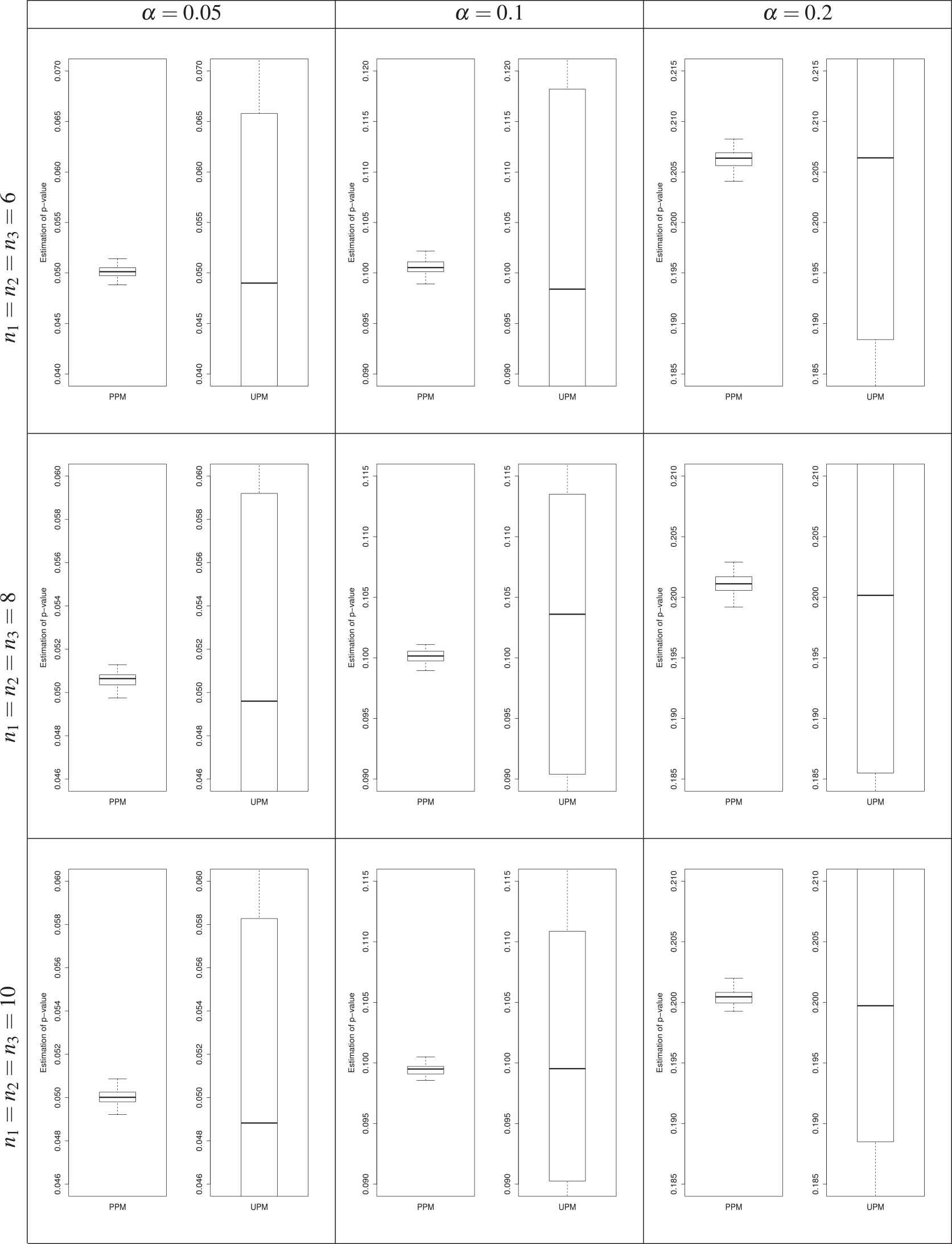
Boxplots of the estimated p-values by PPM and UPM in three cases (n1;n2;n3): (6,6,6), (8,8,8), (10,10,10). The random samples are generated from the skew-normal distribution. PPM and UPM in each subfigure correspond to the usual permutation method and p^(Fsnull(Z);fα).

Heterogeneity of the variance effect on the condition (5): Here, we address an important goal, namely the investigation of the effect of heterogeneity of variance on condition (5). We assume normal distributions for the underlying variables with zero means and the different values in the variances, σ=0.5,1, and 3. The results are shown in Table 3. We can see that the obtained p-values through the AD-test are sufficiently large to satisfy the condition (5).

Sample Sizes n1,n2,n3 Nμ,σ p-value
4,4,4 0,0.5,0,1,0,3 0.694
30,30,30 0,0.5,0,1,0,3 0.549

AD, Anderson–Darling; The null hypothesis is that two samples come from the common distribution.

Table 3

The estimated p-value by AD-test, under heterogeneity of variances.

4.2. Real Data Sets

We have applied our method to two types of microarray data. The first study [13] is aimed to investigate the effectiveness of the processes of brain aging in increasing of Alzheimer's disease. Gene expression values were measured for 30 male rats equally allocated to three groups: aged, mid-aged, and young. For technical reasons, one chip in the young group was lost. We used the updated database since 2014, comprising the measured values of 8799 probe sets on each of the 29 rats and employed the RMAexpress software to calculate the normalized data. Table 4 shows the results. The number of genes identified as differentially expressed is 1081 under a one-way ANOVA, compared with 1098 and 948 obtained using UPM and PPM, respectively.

Method The Number of Detected Genes
Oneway ANOVA 1081
UPM 1098
PPM   948

ANOVA, analysis of variance; UPM, Usual Permutation Method; PPM, Proposed Permutation Method.

Table 4

The number of detected genes as differential gene expression through three methods: one-way ANOVA, UPM, and PPM for the male Fischer rats.

The second example, aimed to identify the reasons for preconceptional endometrial deregulations within in vitro fertilization (IVF) and intracytoplasmic sperm injection (ICSI) [23]. The study investigated whether there is any relation between preconceptional endometrial deregulations and the two events, implantation failures (IFs) and recurrent miscarriages (MSs), when IVF/ICSI is utilized. Three groups are thus considered: a fertile control group comprising women who have had at least one birth, and two test groups comprising women with IF and IM, respectively. Each group contained five subjects. In total, the gene expression values of 22482 genes related to 54675 probe sets were measured. The data were normalized by RMA software. The results of UPM and PPM analysis of this data set are presented in Table 5. Based on a nominal value α=0.01, the RAM-seq software detected 4894 genes with differential expression, compared with 1183 and 321 genes detected by UPM and PPM, respectively.

Method The Number of Detected Genes
Oneway ANOVA 4894
UPM 1183
PPM   321

ANOVA, analysis of variance; UPM, Usual Permutation Method; PPM, Proposed Permutation Method.

Table 5

The number of detected genes as differential gene expression through three methods: one-way ANOVA, UPM, and PPM for the preconceptional endometrial deregulations.

5. CONCLUSIONS

In this paper, we first introduced a new permutation F-test to test the null hypothesis of equal means, for multiple testing with three or more groups. We then modified this test statistic to a null statistic which estimates the corresponding p-values more accurately. We presented several scenarios to evaluate the performance of our procedure for various α and the sample sizes. In the case studies, we confined our attention to three independent groups, although the simulation results clearly illustrate that our methodology performs well under a much wider set of scenarios. The new method is shown to produce p-values with the median much closer to the true α and with a smaller IQR, compared with the usual permutation method.

CONFLICT OF INTEREST

The authors declare they have no conflicts of interest.

ACKNOWLEDGMENTS

The comments of an associate editor and reviewers improved the manuscript significantly. We wish to express our appreciation to them. Thanks are due to our colleague Professor M. Ebrahimi, who assisted in extracting the real data sets. We are also thankful to Dr. S. K. Ghoreishi for his comments.

REFERENCES

Journal
Journal of Statistical Theory and Applications
Volume-Issue
18 - 4
Pages
439 - 449
Publication Date
2019/12/27
ISSN (Online)
2214-1766
ISSN (Print)
1538-7887
DOI
10.2991/jsta.d.191217.001How to use a DOI?
Copyright
© 2019 The Authors. Published by Atlantis Press SARL.
Open Access
This is an open access article distributed under the CC BY-NC 4.0 license (http://creativecommons.org/licenses/by-nc/4.0/).

Cite this article

TY  - JOUR
AU  - Mohsen Salehi
AU  - Adel Mohammadpour
AU  - Kerrie Mengersen
PY  - 2019
DA  - 2019/12/27
TI  - A New F-Test Applicable to Large-Scale Data
JO  - Journal of Statistical Theory and Applications
SP  - 439
EP  - 449
VL  - 18
IS  - 4
SN  - 2214-1766
UR  - https://doi.org/10.2991/jsta.d.191217.001
DO  - 10.2991/jsta.d.191217.001
ID  - Salehi2019
ER  -