1. INTRODUCTION

Wood is extensively used for furniture, building construction and paper production [1]. There are various types of wood and each of them has different attributes with regard to its formation, thickness, color and texture [2]. These varying characteristics defines their ideal usages and economic values [3]. As the price and characteristics of every wood species differs, misclassification may cause financial losses. Hence, there is a need to identify different wood species accurately.

Conventionally, the recognition of wood species is performed manually by human subjects [4]. However, this practice is time and cost consuming to the lumber industry. Hence, several automatic wood species recognition systems have been developed [1,2,5,6]. The efficiency of automatic wood recognition systems can be improved by using superior quality microscopy images which are commonly enhanced to improve the rate of successful wood species recognition. Nevertheless, the image enhancement processes consume extra computational time, and could cause a checkerboard artefact to the wood images [7]. In addition, the dusty and dark environment in timber factories could degrade the quality of the image acquired [8]. Thus, an appropriate Image Quality Assessment (IQA) algorithm is required to assess the acquired wood images prior to feeding it to any automatic wood recognition system.

Image quality assessment can be categorized into subjective and objective evaluations. Subjective evaluation is the scores given by human subjects based on their judgment on the image quality. While, objective evaluation is done based on numerical methods to determine the quality of the images. Even though, subjective evaluation is the benchmark of IQA, it is impracticable in an industrial environment as it is time and cost consuming. Therefore, it is necessary to develop an objective evaluation procedures that is capable to imitate subjective IQA evaluation [9].

Objective evaluation can be categorized into Full-Reference-IQA (FR-IQA) [10–15], Reduced Reference-IQA (RR-IQA) [16,17] and No-Reference/Blind IQA (NR-IQA) [18–20]. FR-IQA uses the reference image fully to assess the images [10–15] whereas RR-IQA uses the reference images partially [16,17]. In contrast, NR-IQA assesses an image without using a reference image [18–21]. NR-IQA is the most appropriate algorithm to evaluate the quality of the wood images as it may be impossible to obtain high quality images in the dusty and dark setting of lumber factories. Therefore, we propose the Gray Level Co-Occurrence Matrix (GLCM) and Gabor features-based NR-IQA, GGNR-IQA algorithm to evaluate wood images.

The GLCM and Gabor features are widely used in wood species recognition system [5,22–24]. The proposed GGNR-IQA algorithm is compared with a commonly utilized NR-IQA, Blind/Referenceless Image Spatial Quality Evaluator (BRISQUE) [18], and FR-IQAs namely, Structural Similarity Index (SSIM) [10], Multiscale SSIM (MS-SSIM) [10], Feature Similarity (FSIM) [11], Information Weighted SSIM (IW-SSIM) [12] and Gradient Magnitude Similarity Deviation (GMSD) [13]. There is significant difference between the proposed GGNR-IQA between the BRISQUE. Technically, BRISQUE is generalized to evaluate natural images and is not suitable to assess the wood images while the proposed GGNR-IQA is trained to assess the wood images. The performances of the GGNR-IQA, BRISQUE and FR-IQAs are evaluated by using the Pearson Linear Correlation Coefficient (PLCC) and Root Mean Squared Error (RMSE) computed between the human Mean Opinion Scores (MOS) and the algorithms.

2. MATERIALS AND METHODS

2.1. Training and Testing Database

An Support Vector Machine Regression (SVR) model is trained with the 44 features of GLCM and Gabor calculated for normalized wood images with the human MOS which are obtained from the subjective evaluation for wood images. The MOS, GLCM and Gabor features are utilized as the training and testing database to obtain an optimized SVR model. The SVM model is used widely in modelling IQA metric as it is capable to handle high-dimensional data exist along with a corresponding lack of knowledge of the underlying distribution. Even with a relatively small sample size, SVMs have the benefit of not being constrained by distributional assumptions, other than that the data are independent and identically distributed [25].

2.1.1. Wood images

Ten wood images from various wood genus, as shown in Figure 1 were chosen. The images were acquired from a wood database: https://www.wood-database.com/ [26]. The images were converted to grayscale and the pixel values were normalized to the range 0–255 for ease of applying the same levels of distortion across all the reference images. The images consisted of a matrix of 600 × 600 pixels, corresponding to resolution of 360,000 and an image area of 9525 cm². The 10 reference images were distorted by Gaussian white noise and motion blur. These two types of distortions usually occur in the industrial setting. Generally, the wood images are exposed to Gaussian white noise due to the poor illumination and heat in the lumber mill while acquiring the wood images [8,27]. On the other hand, wood images are exposed to motion blur when there is a relative motion between the wood slice and camera [6].

Figure 1

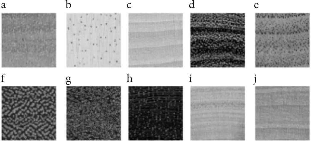
Ten wood images used as reference images (a) Turraeanthus africanus, (b) Ochroma pyramidale, (c) Tilia americana, (d) Cordia spp., (e) Juglans cinerea, (f) Vouacapoua americana, (g) Dipterocarpus spp., (h) Swartzia cubensis, (i) Cordia spp., (j) Cornus florida.

These distortions degrade the quality of the wood images where the features of the pores on the wood texture may not be discerned. Hence, this may lead to misclassification of the wood genus as the feature extractor may not obtain distinctive features from the wood images efficiently [28]. Nine modulations of Gaussian white noise with standard deviation, σ_GN and motion blur with standard deviation, σ_MB were added to the reference images, i.e.: σ_GN = 10, 20, 30, 40, 50, 60, 70, 80 and 90 for Gaussian white noise and σ_MB = 2, 4, 6, 8, 10, 12, 14, 16 and 18 for motion blur.

2.1.2. GLCM and gabor features

First, Mean Subtracted Contrast Normalized (MSCN), Iˆ(m,n) is calculated from the wood image, I(m,n) using Equation (1) [18]:

Iˆ(m,n)=I(m,n)−μ(m,n)σ(m,n)+1 (1)

where μ(m,n) and σ(m,n) denote the mean and variance of wood image, I(m,n), respectively, m ∈ 1, 2, ..., M, n ∈ 1, 2, ..., N are spatial indices while M represents the height and N represents width of image, I(m,n).

The mean, μ(m,n) and variance, σ(m,n) of the wood image are computed using Equations (2) and (3), respectively [18]:

μ(m,n)=∑k=−KK∑l=−LLwk,lIk,l(m,n) (2)

σ(m,n)=∑k=−KK∑l=−LLwk,l(Ik,l(m,n)−μ(m,n))2 (3)

Where w={wk,l|k=−K,…,K,l=−L,…,L} is a 2-dimensional (2D) circularly-symmetric Gaussian weighting function that is sampled out to three standard deviations and rescaled to unit volume, and K and L represent the window sizes.

The MSCN coefficients, Iˆ(m,n) highlights the main features of the wood images such as pores and grains, with few low-energy residual object boundaries [21]. Therefore, the MSCN is used to compute the GLCM and Gabor features instead of the image, I(m,n). Next, two types of features namely, GLCM and Gabor features were incorporated in this study.

2.1.2.1. GLCM features

The GLCM depicts second order statistical analysis of an image by analyzing how often the pairs of pixels which consist of specific values and spatial relationship take place in an image. The probability, p(m, n) is computed using Equation (4) [29]:

p(m,n)={C(m,n)|(d,θ)} (4)

where d is the inter-pixels displacement distance, θ denotes orientation and C(m,n) denotes the frequency of gray level occurrence in MSCN of the image, Iˆ(m,n). Four statistical textures such as contrast, correlation, energy, and homogeneity were extracted from the GLCM matrix.

Contrast calculates the local variations in the GLCM and is defined as Equation (5) [29]:

Contrast=∑m,n|m−n|2p(m,n) (5)

Correlation computes the joint probability occurrence of the specified pixel pairs and is defined as Equation (6) [29]:

Correlation=∑m,n(m−μm)(n−μn)p(m,n)σmσn (6)

Energy calculates the sum of squared components in the GLCM. It is also known as uniformity or the angular second moment. The energy parameter is computed as Equation (7) [29]:

Energy=∑m,np(m,n)2 (7)

Homogeneity calculates the closeness of the distribution of elements in the GLCM to the GLCM diagonal and is computed as Equation (8) [29]:

Homogeneity=∑m,np(m,n)1+|m−n| (8)

These four parameters were computed at four directions, 0°, 45°, 90° and 135° and this form 16 GLCM features.

2.1.2.2. Gabor features

The 2D Gabor function which represents the spatial summation properties of simple cells in the visual cortex and it is defined as Equation (9) [30]:

g(x,y;λ,θ,ψ,σ,γ)=exp(−x′2+γ2y′22σ2)cos(2πx′λ+ψ) (9)

where

x′=x cos θ+y sin θ (10)

y′=−x sin θ+y cos θ (11)

λ denotes the wavelength of the sinusoidal factor, θ denotes the orientation of the normal to the parallel stripes of a Gabor function, ψ represents the phase offset, σ represents the standard deviation of the Gaussian envelope and γ represents the spatial aspect ratio.

The computational models of 2D Gabor filters are defined in Equations (12) and (13) [30]:

he=g(x,y)cos(2πf(xcosθ+ysinθ)) (12)

ho=g(x,y)sin(2πf(xcosθ+ysinθ)) (13)

where h_e and h_o represents the even symmetric and odd symmetric Gabor filters, respectively and g(x,y) represents the isotropic Gaussian function and is computed as Equation (14) [30]:

g(x,y)=12πσ2exp(−x′2+y′22σ2) (14)

And the spatial frequency response of the Gabor functions, f is as shown in Equation (15) [30]:

f=N/P (15)

where N denotes the size of the kernel and P denotes period in pixel.

In this study, wavelength, λ is in increasing powers of two starting from 4/2 up to the hypotenuse length of the input image [31] and this produces seven Gabor features. The seven Gabor features were then computed in four orientations, 0°, 45°, 90° and 135°, similar to the GLCM computations. This forms 28 features Gabor features. In total, the 16 GLCM and 28 Gabor features were combined and this forms 44 features. These 44 features were calculated using the MSCN coefficients, Iˆ(m,n) and are used to train SVR.

2.1.3. MOS

The MOS values were obtained from subjective evaluation participated by 10 students aged between 20 and 25 years from Manipal International University (MIU), Malaysia. The evaluation was carried out as per the procedures suggested in Rec. ITU-R BT.500-11 [32] where it was performed in an office environment using a 21-inch LED computer screen.

Simultaneous double stimulus for continuous evaluation approach was used in this evaluation [32,33] where the reference and distorted images are shown side-by-side on the computer screen and each subject compares the quality of the images displayed on the right side with its reference image (left side) to evaluate the displayed image.

The score given by the human subjects are either Excellent (5), Good (4), Fair (3), Poor (2) or Bad (1) for each image displayed. The evaluation process takes 15–20 min for each subject. The scores obtained from the subjects were averaged to convert them to the MOS [34]. These MOS values are also used to train SVR.

2.1.4. Support vector machine regression

∈-Support Vector Machine Regression (SVR) [35] is trained using MOS and 44 GLCM and Gabor features of wood images in this study. The 44 image features (GLCM and Gabor features) calculated for the wood images are mapped to the MOS values of the corresponding wood images. The 44 GLCM and Gabor features and MOS of wood images were randomly split into training and testing sets where 80% of the 44 features and MOS values were used to train the SVR model to obtain an SVR model with optimized parameters and 20% were utilized to evaluate the optimized SVR model. There was no overlap between the training and testing data to ensure a fair prediction of quality scores. Several experiments were performed on the training and testing data split (70% for training and 30% for testing, 80% for training and 20% for testing and 90% for training and 10% for testing). When a higher percentage of data (90%) for training procedure was tested, the model performance only increased slightly. However, the computation time is longer. A lower percentage of data (70%) for training procedure was tested but the performance of the model decreased. Hence, 80% of data was used for training and 20% of data was used for testing the model.

The flow diagram of the proposed GGNR-IQA is shown in Figure 2. The performance of GGNR-IQA was evaluated using PLCC [36] and RMSE [37] calculated between 1000 iterations were performed on the training and testing of the SVR model to obtain an optimized SVR model. The cost parameter, C, and width parameter, g, of the optimized SVR model are 32,768 and 0.125, respectively.

Figure 2

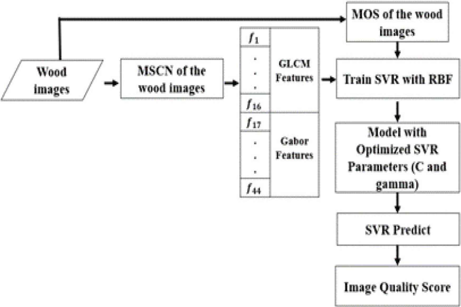
Flow diagram of the proposed GGNR-IQA.

3. RESULTS AND DISCUSSION

The efficiency of the GGNR-IQA was further assessed using a second dataset which was generated from the same wood image database [26]. This second dataset was produced using 10 reference images acquired from 10 various wood genus as shown in Figure 3.

Figure 3

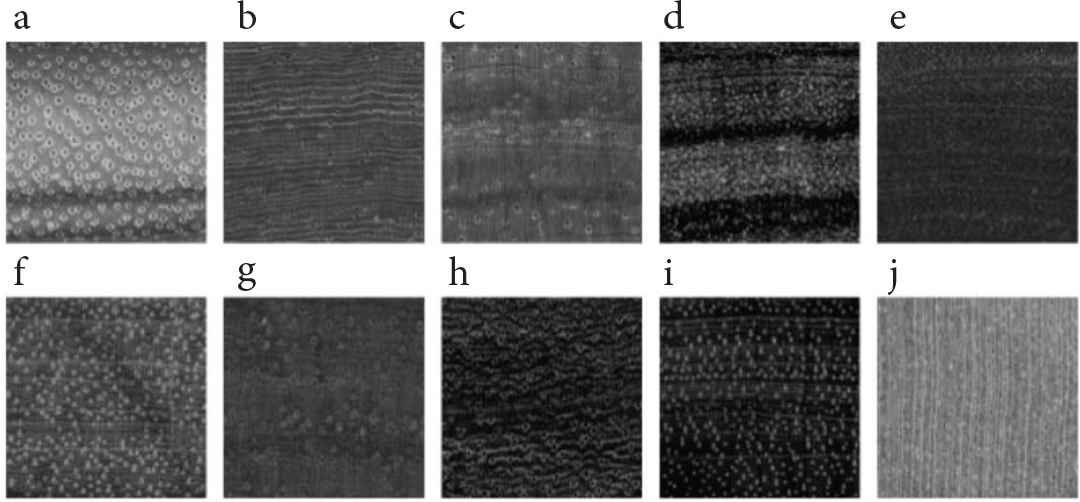
Reference wood images in the second dataset (a) Julbernardia pellegriniana, (b) Dalbergia cultrate, (c) Dalbergia retusa, (d) Dalbergia cearensis, (e) Guaiacum officinale, (f) Swartzia spp., (g) Dalbergia spruceana, (h) Dalbergia sissoo, (i) Swartzia benthamiana and (j) Euxylophora paraensis.

These reference images were added with the similar distortion type (Gaussian white noise and motion blur) and modulations as the training and testing database. This means that the second dataset includes 10 reference images and 180 distorted images.

3.1. Relationship between MOS and Quality of Image with Different Distortion Modulations

Figure 4a and 4b shows the correlation between MOS and nine distortion modulations of Gaussian white noise and motion blur. Lower MOS values show lower image quality which is caused by higher distortion modulation. On the other hand, higher MOS values represent higher image quality which is generated by lower distortion modulation. Based on Figure 4a and 4b, the MOS decreases as the distortion modulation increases. This means that all the human subjects could discern the images distorted with the various modulations of Gaussian white noise and motion blur.

Figure 4

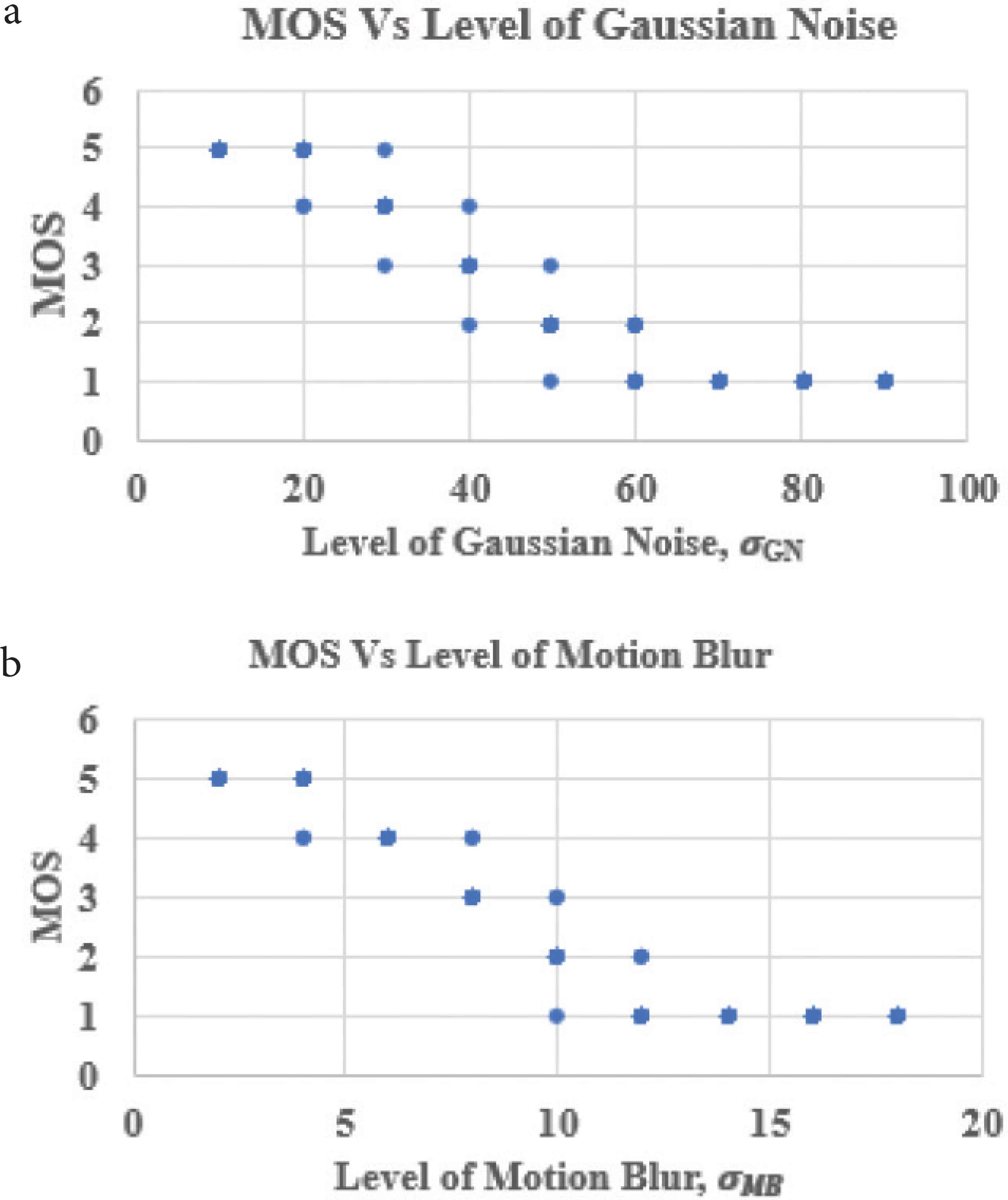
Scatter Plot of MOS versus nine distortion modulations of (a) Gaussian white noise and (b) motion blur.

3.2. Correlation between GGNR-IQA, BRISQUE and FR-IQAs Algorithms and MOS

The PLCC and RMSE values calculated between MOS and the proposed GGNR-IQA metric, BRISQUE and the five FR-IQA metrics are shown in Figures 5 and 6, respectively. The most suitable IQA for wood images is expected to have the highest PLCC and lowest RMSE values. Figure 5 shows that the PLCC values obtained for the GGNR-IQA for Gaussian white noise, motion blur and the overall database are the highest compared to the BRISQUE and FR-IQAs. This shows that the GGNR-IQA algorithm outperforms BRISQUE and all the five FR-IQAs. This is further proved with the lowest RMSE values for the proposed metric compared to BRISQUE and all the five FR-IQAs as shown in Figure 6.

Figure 5

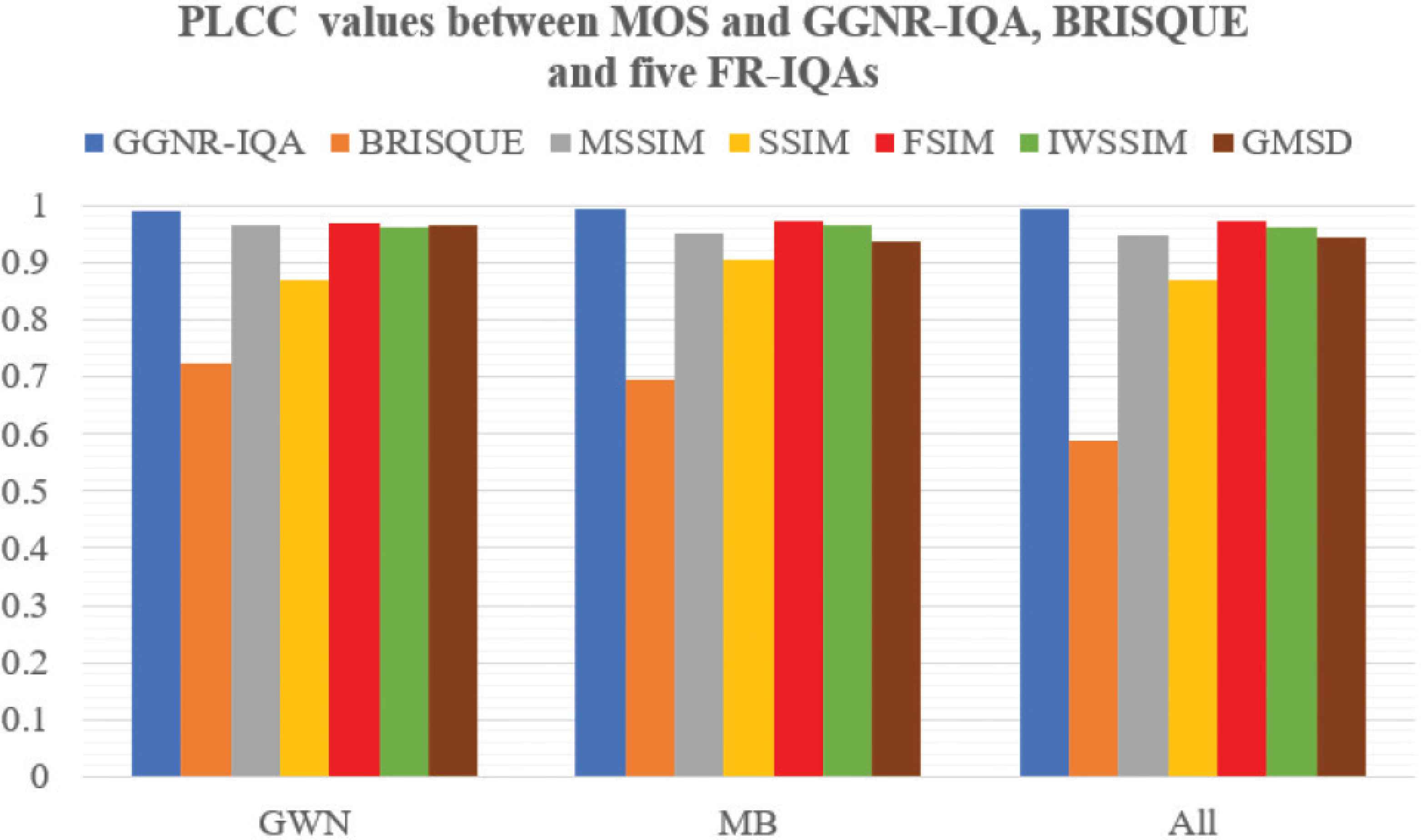
PLCC values between GGNR-IQA, BRISQUE, FR-IQAs and MOS.

Figure 6

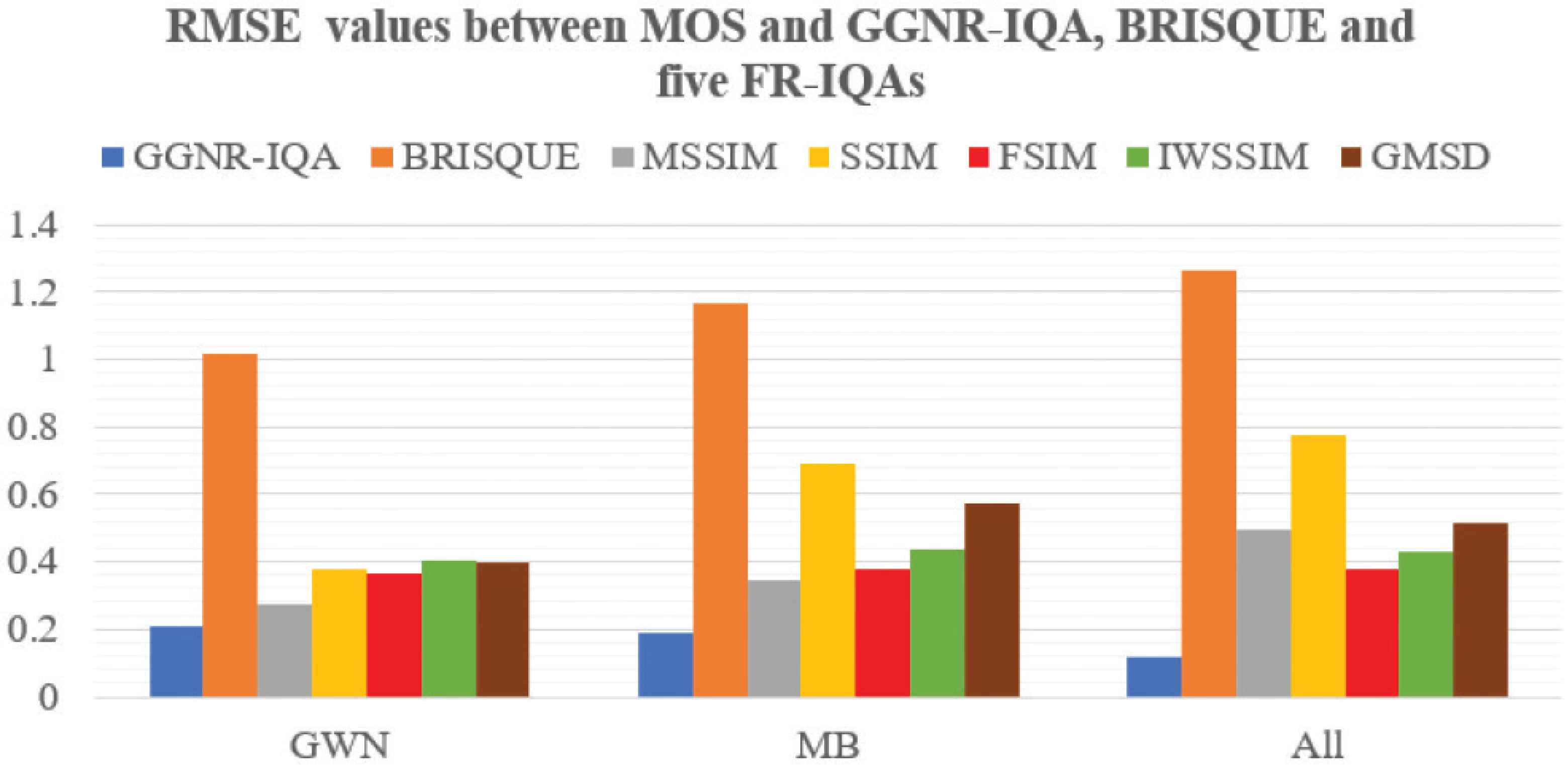
RMSE values between GGNR-IQA, BRISQUE, FR-IQAs and MOS.

4. CONCLUSION

A NR-IQA algorithm, GGNR-IQA was proposed to assess wood images prior to feeding the image to wood species classification and recognition system. The proposed GGNR-IQA algorithm was trained using GLCM, Gabor features and MOS obtained from wood images. The performance of the GGNR-IQA algorithm was assessed by comparing the PLCC and RMSE values calculated between GGNR-IQA, BRISQUE, five FR-IQA algorithms and MOS. PLCC and RMSE values showed that the GGNR-IQA algorithm outperforms BRISQUE and all the five FR-IQAs. This shows that the GGNR-IQA algorithm could assess the quality of wood images accurately. In addition, the proposed GGNR-IQA algorithm would not require a distortion free reference image to determine the quality of the wood images. This is beneficial especially when it is impossible to obtain a distortion free reference image in the dusty environment of lumber mill.

CONFLICTS OF INTEREST

The authors declare they have no conflicts of interest.

AUTHORS INTRODUCTION

Ms. Heshalini Rajagopal

She received her Master’s degree from the Department of Electrical Engineering, University of Malaya, Malaysia in 2016. She has passed her PhD Viva Voce in University of Malaya, Malaysia recently. She received the B.E. (Electrical) in 2013 and MEngSc in 2016 from University of Malaya, Malaysia. Currently, she is a lecturer in Manipal International University, Nilai, Malaysia. Her research interests include image processing, artificial intelligence and machine learning.

Dr. Norrima Mokhtar

She received the B.Eng. degree from University of Malaya, the M.Eng. and the PhD degree from Oita Univerity, Japan. She is currently a senior lecturer in the Department of Electrical Engineering, University of Malaya. Her research interests are signal processing and human machine interface.

Dr. Anis Salwa Mohd Khairuddin

She received PhD in computer engineering at Universiti Teknologi Malaysia (UTM). She received the B.Eng. (Hons) Electrical and Electronics Engineering from Universiti Tenaga Nasional, Malaysia, in 2007 and Masters degree in computer engineering from Royal Melbourne Institute of Technology, Australia, in 2009. She is currently a Senior Lecturer from University of Malaya. Her current interests include pattern recognition, image analysis, and artificial intelligence.

Dr. Wan Khairunizam

He received his B.Eng. degree in Electrical & Electronic Engineering from Yamaguchi University and PhD in Intelligent Mechanical System Engineering from Kagawa University, Japan in 1999 and 2009 respectively. He is currently an Associate Professor of Mechatronic at School of Mechatronic Engineering, University Malaysia Perlis (UniMAP), Malaysia. His specialties are in Human-Computer Interaction, Intelligent Transportation System (ITS), Artificial Intelligence (AI) and Robotics.

Dr. Zuwairie Ibrahim

He received his B.Eng. (Mechatronics) and M.Eng. (Image Processing) from Universiti Teknologi Malaysia, in 2000 and 2002, respectively. In 2006, he has been awarded a PhD (DNA Computing) from Meiji University, Japan. He is currently an Associate Professor in the Faculty of Electrical and Electronic Engineering, Universiti Malaysia Pahang. His research interests include computational intelligence, image processing, and unconventional computation such as molecular or DNA computing.

Dr. Asrul Bin Adam

He received the B.Eng. and M.Eng. degrees in Electrical-Mechatronics and Electrical Engineering from Universiti Teknologi Malaysia (UTM), Malaysia, in 2009 and 2012, respectively. He completed his PhD in Signal and System from Faculty of Engineering, University of Malaya in 2017. He currently works as lecturer at Faculty of Manufacturing Engineering, Universiti Malaysia Pahang, Malaysia. His research interests include biomedical signals processing, artificial intelligent, machine learning, and optimization.

Dr. Wan Amirul Bin Wan Mohd Mahiyidin

He received the M.Eng. degree from the Imperial College London in 2009, the M.Sc. degree from University of Malaya in 2012, and the PhD degree from University of Canterbury in 2016. He is currently a senior lecturer at the Department of Electrical Engineering, University of Malaya. His research interests are multiple antennas system, cooperative MIMO, channel modelling and positioning system.