
Kinematic Modeling and Simulation of Dual-Arm Robot
- DOI
- 10.2991/jrnal.k.210521.013How to use a DOI?
- Keywords
- Dual-arm robots; real-time; inverse kinematics; simulation
- Abstract
In recent years, dual-arm robots have attracted more and more attention due to their advantages such as strong cooperation ability and high flexibility. With the improvement of real-time requirement of dual-arm cooperation, the inverse kinematics solution of robot becomes a key problem to be solved urgently. To solve the time-consuming problem of inverse kinematics of robot arm, a closed inverse kinematics solution algorithm for humanoid dual-arm robot was proposed. The effectiveness of the algorithm was verified by simulation.
- Copyright
- © 2021 The Authors. Published by Atlantis Press B.V.
- Open Access
- This is an open access article distributed under the CC BY-NC 4.0 license (http://creativecommons.org/licenses/by-nc/4.0/).
1. INTRODUCTION
Humanoid dual-arm robot is a kind of bionic robot designed by imitating the shape, structure and function of human body. It can work with both hands cooperatively just like human. The inverse kinematics of manipulator mainly includes geometric method, analytical method and numerical method. The geometric method is a special case of analytic method in some cases, and its applicability is weak [1,2]. Analytical inverse kinematics of the manipulator can efficiently obtain all the inverse solutions of the manipulator in the desired position, but the manipulator must satisfy the Piper criterion [3]. The numerical method has no special requirements for the joint number and structure of the manipulator, but it needs to be solved through continuous iteration, which not only takes a long time, but the average calculation error is also 10 times that of the analytical method [4,5].
Because it takes a long time to meet the accuracy requirement and solve the problem of manipulator inverse kinematics solution, the analytical solution is adopted. In Section 2, a closed inverse kinematics algorithm is proposed for the humanoid robot arms. The algorithm is used for simulation analysis in Section 3. And we verify the effectiveness of the algorithm in Section 4.
2. KINEMATIC MODELING OF DUAL-ARM ROBOT
2.1. Forward Kinematics
The robot model in this paper is shown in Figure 1. Each arm of the robot has six Degrees of Freedom (DOF). The three axes of the shoulder joint intersect at one point. Because this case conforms to the Piper criterion, there are analytic solutions. In general, the end of the robot meets the Piper criterion, but the shoulder joint of the humanoid robot generally meets the Piper criterion. Although it looks the same, their solutions are different. Taking the shoulder joint as the basic coordinate frame [6], Figure 1 also shows the link coordinate frames of the right arm and its D–H parameters. Where joint i represents the i-th joint of the manipulator, θi is the angle between xi−1 and xi, di is the distance between xi−1 and xi, ai is the distance between zi−1 and zi, αi is the angle between zi−1 and zi. The left arm and the right arm are identical.
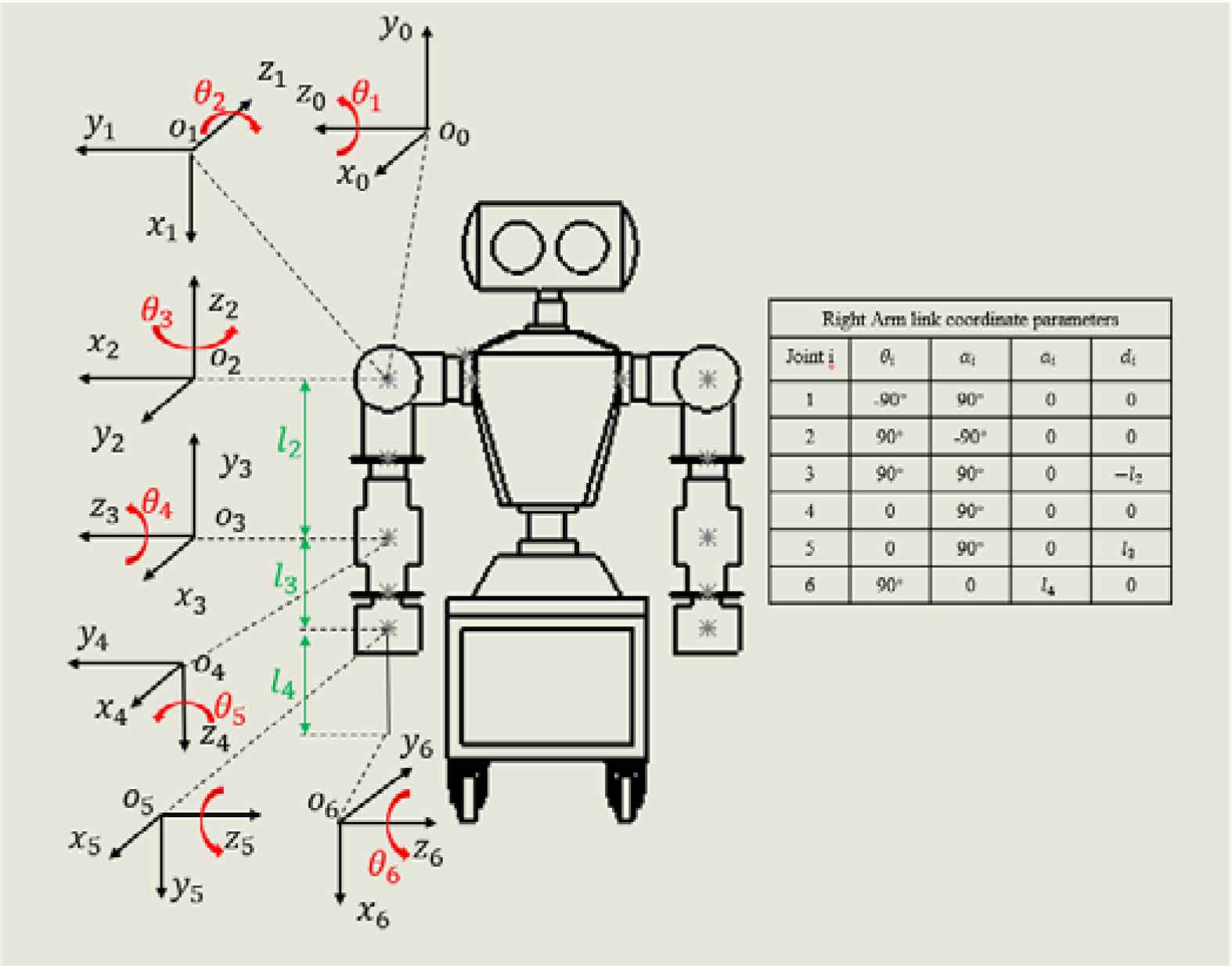
Link coordinate frames of the right arm and its D–H parameters.
The position and orientation of the end-effector can be obtained by chain-multiplying the six link-transformation matrices together to obtain the spatial displacement of the sixth coordinate frame with respect to the base coordinate frame:
2.2. Inverse Kinematics
We take the inverse of both sides of Equation (1). The new matrix T′ is
We can obtain an equation that we label as E2 equation by moving the link transformation matrix 5A6 to the left-hand side of Equation (2).
The left-hand side of E2 is
And the right-hand side of E2 is
Where Si ≡ sin θi, Ci ≡ cos θi, Sij ≡ sin(θi + θj), Ci ≡ cos(θi + θj), and lLi are geometric link parameters in Figure 1. By comparing the elements (1, 4), (2, 4) and (3, 4) of the EL2 and ER2, we can obtain C4 and then S4 from C4, and from which we can find the joint solution for θ4. we can solve θ5 when we have solved θ4. Similarly, we can solve θ6 when we have solved θ4 and θ5.
To solve for the remaining joint angles, we can move the link transformation matrix 3A4 4A5 to the left-hand side of Equation (3). And we can obtain an equation that we label as E4 equation.
The left-hand side of E4 is
And the right-hand side of E4 is
By comparing the element (2, 3) of EL4 and ER4, we get C2 and then S2, and the joint solution θ2 from them,
By comparing the elements [(1, 3) (3, 3)] and [(2, 1) (2, 2)], we can find the joint solution θ3 and θ1,
The solution of the six joints is obtained by the above procedure. The left arm is exactly the same as the right arm for the solution.
3. DUAL-ARM ROBOT MODELING BASED ON SIMSCAPE
3.1. Model Building
In this paper, the dual-arm robot simulation model mainly includes three parts, namely the trajectory planning joint angle input module, the robot body module and the output measurement module. Its Simscape Multibody model is shown in Figure 2.
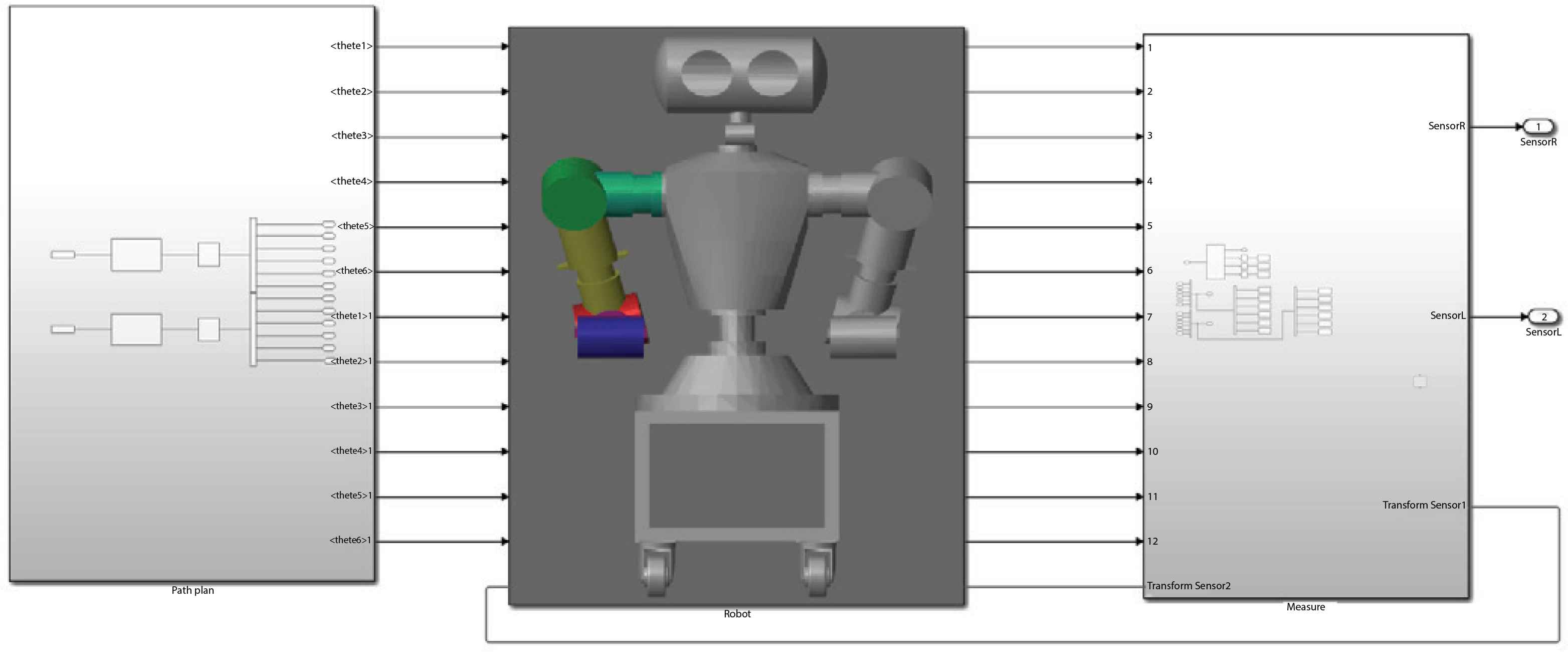
Dual-arm robot simulation model.
3.2. Establishment of Joint Angle Input Module for Trajectory Planning
We plan the trajectory of space in Cartesian coordinates. After solving the inverse kinematics function, we can obtain the angles of each joint. Then we output these angles to the various joints of the arm. The joint angle input model for trajectory planning is shown in Figure 3.
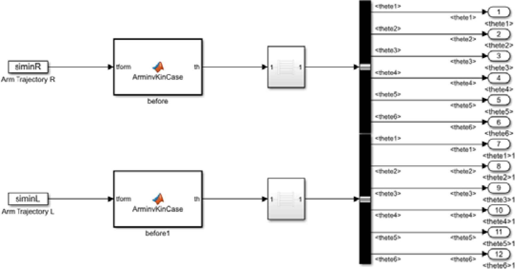
The joint angle input model for trajectory.
3.3. Establishment of Robot Ontology Module
Figure 4 shows the robot ontology module. It includes world coordinate frame and robot ontology. The robot has two arms. Each arm has six DOF, including three DOF for shoulder joint, one DOF for elbow joint and two DOF for wrist joint.
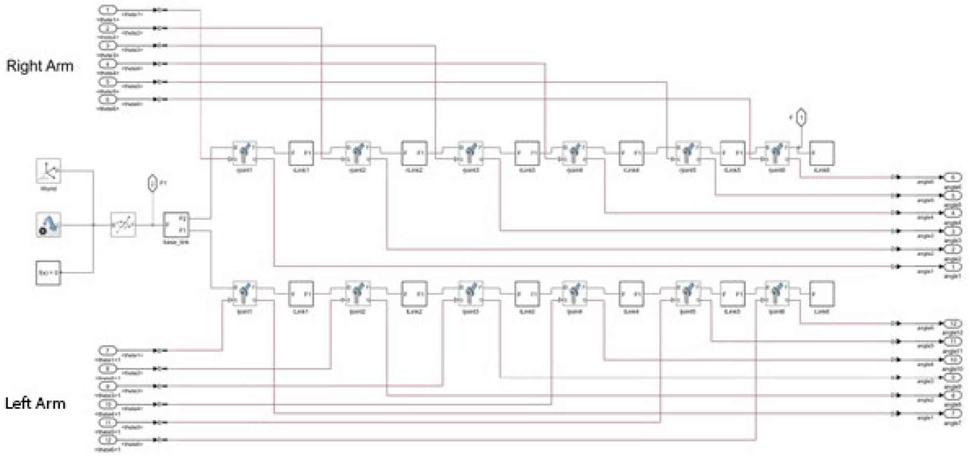
The robot ontology module.
3.4. Establishment of Output Measurement Module
The output measurement module shown in Figure 5 can measure the rotation angle of each DOF. Through this module, we can also obtain the displacement of the terminal coordinate frame of the manipulator relative to the base coordinate frame.
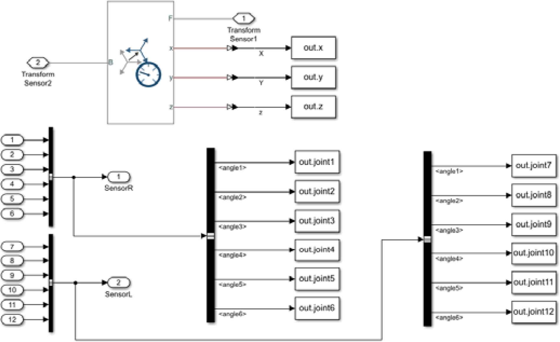
The output measurement module.
4. SIMULATION VERIFICATION AND ANALYSIS
4.1. Simulation Process
The robot first raised their arms and then approached each other. The entire process is shown in Figure 6.
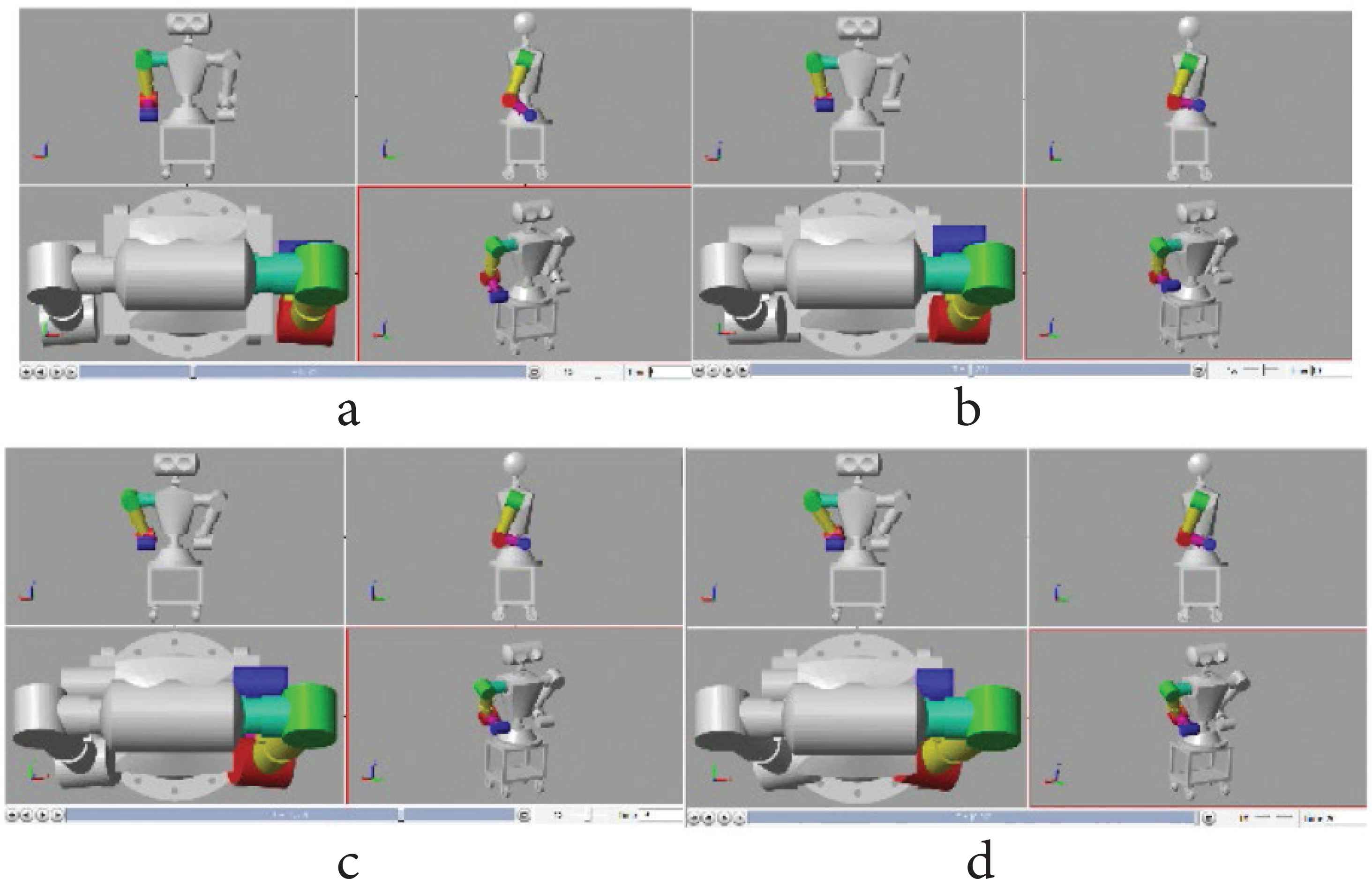
Simulation diagram of each moment. (a) t = 5 s. (b) t = 10 s. (c) t = 15 s. (d) t = 20 s.
4.2. The Motion Angles of Each Joint
Figure 7 shows the motion angles of each joint of the manipulator. At the initial moment, the angle of each joint is 0 radian, and at about 10 s, the robotic arms begin to approach each other. The angle of each joint is continuous in the whole process, which proves that the inverse kinematics solution algorithm in this paper can solve the analytic solution effectively.
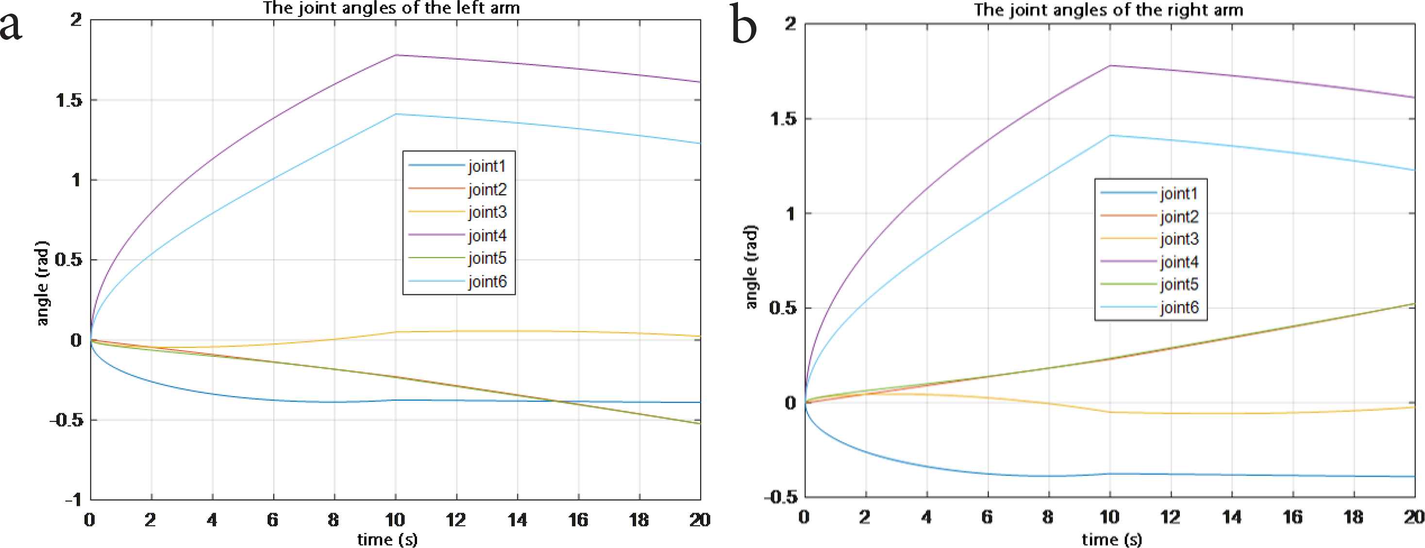
The motion angles of each joint of the (a) left and (b) right arms.
5. CONCLUSION
In this paper, the kinematics modeling of dual-arm robot is carried out. We present an analytical solution method for six DOF dual-arm robot for each arm. Simulation results show that the proposed method is effective. In the future, it will be applied to the arm trajectory planning of the robot.
CONFLICTS OF INTEREST
The authors declare they have no conflicts of interest.
ACKNOWLEDGMENT
This work was supported by the Key Research and Development Program (No. M18GY300021).
AUTHORS INTRODUCTION
Dr. Jiwu Wang
 He is an Associate Professor, Beijing Jiaotong University. His research interests are Intelligent Robot, Machine Vision, and Image Processing.
Mr. Junxiang Xu
 He is a postgraduate in Beijing Jiaotong University. His research interest is Robot Modeling and Simulation.
REFERENCES
Cite this article
TY  - JOUR
AU  - Jiwu Wang
AU  - Junxiang Xu
PY  - 2021
DA  - 2021/06/06
TI  - Kinematic Modeling and Simulation of Dual-Arm Robot
JO  - Journal of Robotics, Networking and Artificial Life
SP  - 56
EP  - 59
VL  - 8
IS  - 1
SN  - 2352-6386
UR  - https://doi.org/10.2991/jrnal.k.210521.013
DO  - 10.2991/jrnal.k.210521.013
ID  - Wang2021
ER  -