
Possible Mechanism of Internal Visual Perception: Context-dependent Processing by Predictive Coding and Reservoir Computing Network
- DOI
- 10.2991/jrnal.k.190531.009How to use a DOI?
- Keywords
- Visual system; perception; predictive coding; reservoir computing; context; nonlinear dynamics
- Abstract
The predictive coding is a widely accepted hypothesis on how our internal visual perceptions are generated. Dynamical predictive coding with reservoir computing (PCRC) models have been proposed, but how they work remains to be clarified. Therefore, we first construct a simple PCRC network and analyze the nonlinear dynamics underlying it. Since the influence of contexts is another important factor on the visual perception, we also construct PCRC networks for the context-dependent task, and observe their attractor-landscapes on each context.
- Copyright
- © 2019 The Authors. Published by Atlantis Press SARL.
- Open Access
- This is an open access article distributed under the CC BY-NC 4.0 license (http://creativecommons.org/licenses/by-nc/4.0/).
1. INTRODUCTION
It is widely known that what we see is not the visual sensory input as it is. Instead, our brains integrate the sensory inputs and reconstruct the internal image in the manner we can easily understand. For example, although the actual visual input is 2D and received by both eyes, what we see is the 3D vision as one image. However, exactly how the internal visual perceptions are generated in the visual cortex has provoked much debate.
The predictive coding is one of the most accepted hypotheses on the internal perception. In the predictive coding framework, a perceived image is not merely the integrated visual sensory input, but the result of the prediction made by the internal generative model. The predictive coding also assumes that the generative model is optimized to minimize the residual error between the prediction and the actual sensory input. In particular, the hierarchical predictive coding model [1] postulates that the top-down signals from the higher-order area carry the predictions of lower-level neural activities, whereas the bottom-up signals from the lower-order area carry the residual errors between the predictions and the actual lower-level activities, so that the ascending signals have much less redundancy.
However, this model is only suitable for static visual inputs and cannot deal with temporally changing visual images, or movies. Then Fukino et al. [2] proposed the Predictive Coding with Reservoir Computing (PCRC) model, which can predict the temporally changing auditory inputs, implementing the generative model by the dynamical reservoir. Furthermore, the hierarchical PCRC models for more complex auditory inputs were proposed by Ara and Katori [3,4].
Here, the reservoir computing [5] refers to a type of the Recurrent Neural Network (RNN) approach with a simple learning strategy. When the reservoir computing networks are trained, only the output connections are modified, and the recurrent and feedback connections are fixed with randomly given values.
However, precisely how these PCRC models [2–4] work largely remains to be clarified. Moreover, these conventional models cannot perceive unlearned inputs. In addition, they are not exactly driven by the prediction error but by the sum of the error and their own prediction, which is equal to the original sensory input.
In this study, therefore, we first modify them and construct a simple one-layer PCRC network exactly driven by the prediction errors, which can perceive even unlearned inputs. Then we analyze the nonlinear dynamics underlying the trained network, in order to clarify the mechanism of the behavior.
The influence of contexts, which refers to situations, goals, and relevant past experiences, is another important factor on the visual perception. For example, even identical sensory stimuli can result in very different perceptions depending on contexts. Indeed, RNN models for context-dependent tasks have been proposed [6].
Therefore, we also construct a PCRC network for a simple context-dependent perception task. We analyze the trained network again, in order to reveal how the network perceives the sensory stimuli on each context. We further construct a PCRC network which can perceive more high-dimensional visual inputs, in order to show that the proposed network can be a possible mechanism of the visual perception. We observe that the mismatch between the context and the type of sensory stimuli induces the perceptual error, which exhibits complex visual features.
2. SIMPLE PCRC
In this section, we construct a simple one-layer PCRC network exactly driven by the prediction errors. We also analyze the nonlinear dynamics underlying the trained network to elucidate how it works.
2.1. Network Architecture and Dynamics
We use a leaky-integrator RNN, defined by the equation:
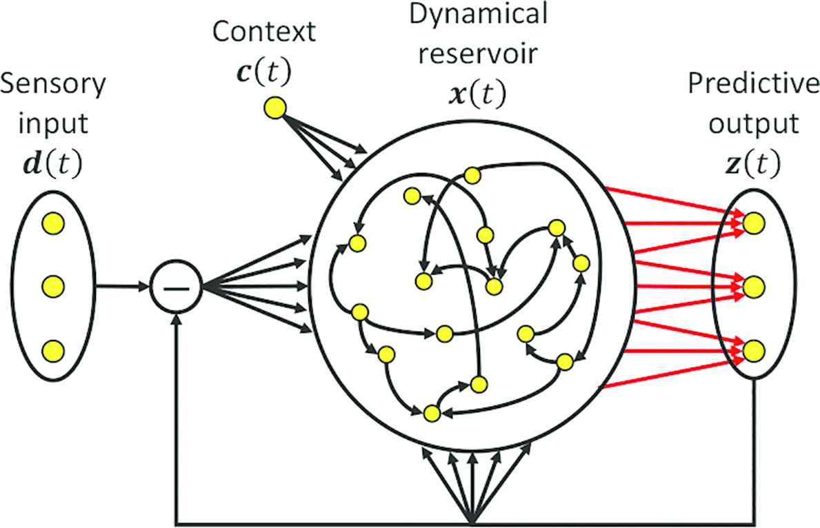
Schematic chart of the one-layer PCRC network architecture. Only the output weights (red) are modified during training.
In order to simulate this dynamics numerically, we introduce the discrete-time version of Equation (1), derived by Euler method:
Throughout this paper, we use N = 1000, g = 1.2, τ = 100 ms, and δ = 10. In this section, we use M = 2 for visibility of the dynamics.
2.2. Task
We present the constant vectors d1,..., dND ∈ ℝM in turn as the sensory inputs to the network, where ND is the number of trials. The network is trained to keep outputting the target di until the next target di+1 is presented, at each ith trial. Each sensory input di is presented for 0.2 s, and its elements are independently and uniformly sampled from [1, 2].
Since the network actually receive the prediction error di – z(t) as the input, it is required to decode this error into the original sensory input di. This corresponds to the framework of the predictive coding.
2.3. Learning Rule
We train WOUT by Fast Order Reduced and Controlled Error (FORCE) learning algorithm [7], which is based on the recursive least square filter. Its update rule is:
In this algorithm, the inverse of P(t) is a running estimate of the autocorrelation matrix of the firing rates r(t) plus a regularization term:
Throughout this paper, we use α = 0.02 and Δt = δ.
2.4. Results and Analysis
We trained the network for 1000 trials. (i.e., ND = 1000). At each trial in the test phase, the sensory input di is presented for 5.0 s. As shown in Figure 2, the training resulted in almost perfect performance. Figure 2 also shows that at the beginning of each ith trial, the prediction error di – z(t) is fed to the network as a sharp pulse, but it immediately decays to zero and the network settles into a fixed point
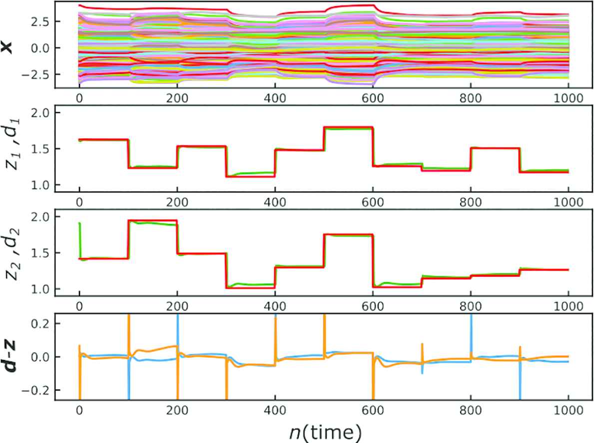
The response of the trained network in the test phase. The 1st row represents the activities of the reservoir x(t), red plots in the 2nd and 3rd row represent the target d(t), green plots in the 2nd and 3rd row represent the output z(t), and the 4th row represents the prediction error d(t) – z(t).
In order to reveal the underling mechanism of this behavior, we analyze the nonlinear dynamics of the trained network. In what follows, we regard the term WIN (d – z) as the external force and separate it from the network’s own dynamics, because of its pulse-like behavior, i.e., we here analyze the dynamics:
Following the approach of Sussillo and Barak [8], we define the scalar function q(x) ≔ |ẋ|2/2, which is near to zero if x is an approximate fixed point, or a slow point. Figure 3a shows that almost all the q values at the end of trials are very low, and the corresponding slow points are located on a 2D-manifold in the phase space. Figure 3a also shows that at the beginning of each ith trial, the pulse-like prediction error di – z(t) drives the trajectory out of the 2D-manifold, but in the subsequent relaxation phase, the trajectory is attracted by the 2D-manifold, and the projection of the trajectory onto the manifold corresponds to the total movement di – di–1.
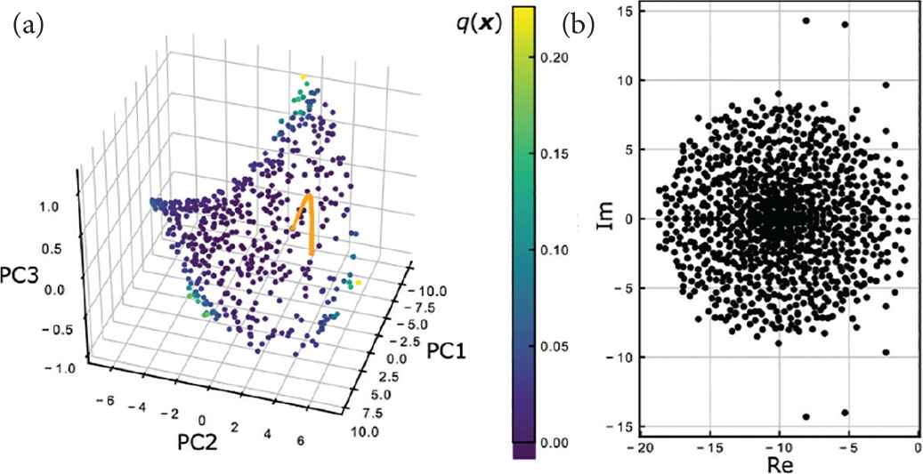
(a) The locations of the slow points
Furthermore, by analyzing the linearized system around each slow point on the 2D-manifold, we uncover the stability of this manifold. Linearizing Equation (9) around the slow point
As for almost all the slow points, the linearized systems around them have only eigenvalues with the negative real part, as shown in Figure 3b. This suggests that almost all the slow points are locally stable, and the 2D-manifold composed of them attracts any trajectories in the vicinity of it. Nevertheless, this manifold attractor is not fully continuous and there is a slow flow on it. Then the trajectory on the manifold is attracted by the specific slow point on the manifold where the output z(t) is near to but not equal to the target di, which leads to the little prediction error shown in Figure 2.
Up to this point, the trained network has exhibited the performance only on the discontinuously changing sensory inputs. Here we show that the same network can also perceive the continuously changing sensory inputs. For example, Figure 4a shows that the network output succeeded in following the sinusoidal input. In this case the network trajectory x(t) keeps travelling around the 2D-manifold in the phase space, as shown in Figure 4b. This behavior results from the balance between the attracting force from the 2D-manifold and the driving force by the prediction error d(t) – z(t). Even in the general case, the same mechanism enables the network to perceive the continuously changing input.
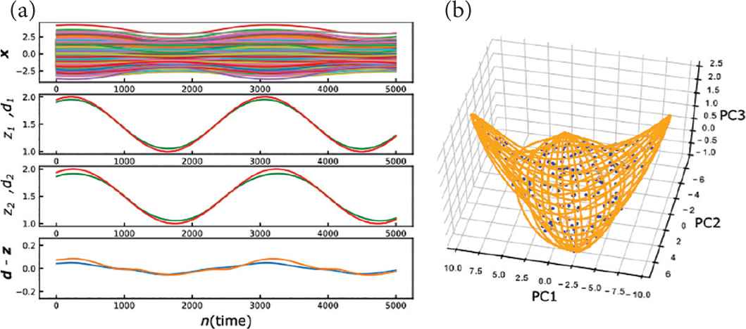
The response of the trained network to a continuously changing sensory input. (a) The activities of the reservoir x(t) (the 1st row), the target d(t) (red plots in the 2nd and 3rd row), the output z(t) (green plots in the 2nd and 3rd row), and the prediction error d(t) – z(t) (the 4th row). (b) The trajectory of x(t) (orange) and the 2D-manifold composed of the stable slow points (blue) in 3D PCA space.
Throughout this section, we have shown the case of M = 2 for simplicity, but the same scenario holds for the case of general M.
3. CONTEXT-DEPENDENT PCRC
In this section, we construct a simple PCRC network for the context-dependent perception task. We also analyze the trained network to elucidate how it switches the processing depending on contexts.
3.1. Network Architecture and Dynamics
We add to Equation (1) the term of the context signal from external modules:
3.2. Task and Learning Rule
We present the constant vectors d1,…,dND ∈ ℝM in turn as the sensory inputs to the network, and train the network to keep outputting each given constant vector until the next target is presented. We also present the context c1 ≔ (0,1)T during the 1st to ND/2th trials, and the context c2 ≔ (1, 0)T during the ND/2+1th to NDth trials, respectively. Each sensory input di is presented for 0.2 s, and its elements are given as
We train WOUT by FORCE learning algorithm used in Section 2.
3.3. Results and Analysis
We trained the network for 1000 trials on each context c1 and c2. (i.e., ND = 2000). At each trial in the test phase, the sensory input di is presented for 1.0 s. As shown in Figure 5a, the training resulted in almost perfect performance, and the pulse-like prediction error drives the network from one slow point to another, as with the context-free case in Section 2. Figure 5b shows that the two different 2D-manifold attractors are formed for the contexts c1 and c2, respectively. This suggests that the network switches its attractor-landscape depending on contexts, and the same mechanism as Section 2 enables the network to perceive the sensory inputs on each context.
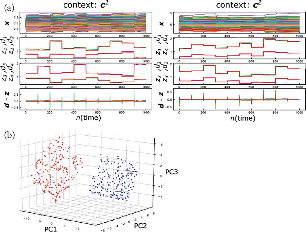
The context-dependent response of the trained network. (a) The activities of the reservoir x(t) (the 1st row), the target d(t) (red plots in the 2nd and 3rd row), the output z(t) (green and purple plots in the 2nd and 3rd row), and the prediction error d(t) – z(t) (the 4th row). (Left: context c1. Right: context c2). (b) The locations of the slow points
We next evaluate the performance of the trained network when the type of the sensory input (
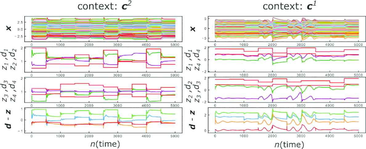
The perceptual errors induced by the context mismatch. (Left:
4. CONTEXT-DEPENDENT PCRC FOR VISUAL DATA
In this section, we construct a context-dependent PCRC network which can perceive more high-dimensional visual inputs, in order to demonstrate that the proposed network can be a possible mechanism of the visual perception. We also observe the complex features of the perceptual error induced by the context mismatch.
4.1. Network Architecture, Task, and Learning Rules
The network architecture and settings follow those of Section 3, except the dimension of the input and output: M = 20.
We use the Mixed National Institute of Standards and Technology (MNIST) data set, which is widely used for handwritten numeral recognition tasks, as the high-dimensional visual sensory stimuli. As the preprocessing, we first compress the MNIST data whose labels are “0” or “1” into 20 dimension, using the Non-negative Matrix Factorization (NMF). We next randomly choose one of the compressed MNIST data as the sensory input di and present it to the network for 0.2 s at each ith trial. At the same time, we present the context c1 if di has “0” label, and the context c2 if di has “1” label, respectively. (i.e., each context represents the category of the visual sensory input). We train the network to keep outputting the presented sensory input di during each trial. In the test phase, we present to the network unlearned compressed MNIST data as the sensory inputs. The trained network is required to form slow points that correspond to even unlearned MNIST data in its phase space.
We use the FORCE algorithm again during training.
4.2. Results and Analysis
We trained the network for 2000 trials on each context c1 and c2. (i.e., ND = 4000). At each trial in the test phase, we present a randomly chosen unlearned MNIST data for 5.0 s as the sensory input di. Figure 7a shows that the training network almost succeeded in perceiving unlearned MNIST inputs, and the pulse-like prediction error drives the network from one slow point to another, as with the case above. Figure 7b shows that the two different manifold attractors are formed for the “0” label and “1” label MNIST inputs respectively, but in the 3D PCA space we cannot observe the actual shapes of these manifolds.
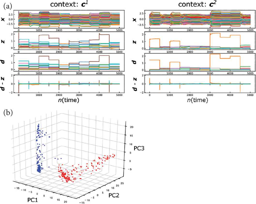
The context-dependent response of the trained network to unlearned MNIST inputs. (a) The activity of the reservoir x(t), the output z(t), the target d(t) and the prediction error d(t) – z(t). (Left: context c1. Right: context c2). (b) The locations of the slow points
We next evaluate the performance of the trained network when the label of the sensory input does not match the context. As shown in Figure 8, the context mismatch keeps the prediction errors apart from zero, but nevertheless the network trajectories settle into slow points.
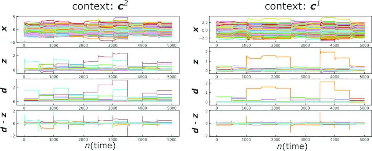
The perceptual errors induced by the context mismatch. (Left: label “0” data are presented on the context c2. Right: label “1” data are presented on the context c1).
We further visualize these errored predictions z at slow points and compare them with the original inputs d, by inversely transforming the output z into the dimension of the original MNIST data, using the matrix generated in NMF. As a result, in the errored predictions, the original sensory inputs and the predictions for the wrong label MNIST image overlap each other, as illustrated in Figure 9.
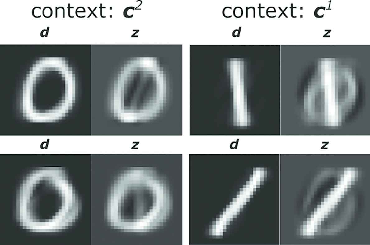
The examples of the visualized comparison between the original inputs d and errored predictions z on the context mismatch. (Left: label “0” data are presented on the context c2. Right: label “1” data are presented on the context c1).
5. DISCUSSION
We first proposed the simple one-layer PCRC network driven by the prediction error, which can perceive even unlearned inputs. We analyzed the nonlinear dynamics underling the trained network, and revealed that the network perceives the sensory stimuli using the low-dimensional manifold attractor in its phase space. Since low-dimensional manifold attractors have also been observed in the trained RNNs in previous studies [6,8,9], it can be a natural strategy for RNNs to use them for the information processing.
Next, we constructed the simple PCRC network for the context-dependent task, and observed that the different attractor-landscape is formed on each context. Throughout this study, we used the PCRC networks with only one layer and assumed the context signals to be fed from the external module, for simplicity. However, the hierarchy plays a key role in the predictive coding framework [1], and how the context signals are generated remains to be clarified. Therefore, it is our future work to build the hierarchical PCRC model composed of the one-layer networks which are analyzed in this study, and incorporate the modules which generate the context signals inside the model.
Finally, we constructed the context-dependent PCRC network for the compressed MNIST data task, and demonstrated that the proposed network can be a possible mechanism of the visual perception. The perceptual errors induced by the context mismatch exhibited complex features, and interestingly, they share some common features with the symptoms of the hallucination in dementia with Lewy bodies [10], in which the patients see other people who are not there on the background which actually exists there. It is also our future work to study the relation between these perceptual errors.
CONFLICTS OF INTEREST
There is no conflicts of interest.
ACKNOWLEDGMENTS
The authors are grateful to T. Kohno for useful discussions. This paper is partially supported by AMED under Grant Number JP18dm0307009, NEC Corporation, and JSPS KAKENHI Grant Number JP16K00246, and also based on results obtained from a project subsidized by the New Energy and Industrial Technology Development Organization (NEDO).
Authors Introduction
Mr. Hiroto Tamura
 He received the B.E. degree of applied mathematics in 2017 from Waseda University, Japan, and the M.E. degree of electronic engineering in 2019 from the University of Tokyo, Japan. Currently, he is PhD Candidate of Graduate School of Engineering, the University of Tokyo. His research interests include computational neuroscience and nonlinear dynamics.
Dr. Yuichi Katori
 He received the PhD degree of science in 2007 from the University of Tokyo, Japan. Currently, he is Associate Professor of Future University Hakodate. His research interests include mathematical modeling of complex systems, computational neuroscience, and brain-like artificial intelligence systems.
Dr. Kazuyuki Aihara
 He received the B.E. degree of electrical engineering in 1977 and the PhD degree of electronic engineering 1982 from the University of Tokyo, Japan. Currently, he is Professor of Institute of Industrial Science, Graduate School of Information Science and Technology, and Graduate School of Engineering, the University of Tokyo. His research interests include mathematical modeling of complex systems, parallel distributed processing with spatio-temporal neurodynamics, and time series analysis of complex data.
REFERENCES
Cite this article
TY  - JOUR
AU  - Hiroto Tamura
AU  - Yuichi Katori
AU  - Kazuyuki Aihara
PY  - 2019
DA  - 2019/06/25
TI  - Possible Mechanism of Internal Visual Perception: Context-dependent Processing by Predictive Coding and Reservoir Computing Network
JO  - Journal of Robotics, Networking and Artificial Life
SP  - 42
EP  - 47
VL  - 6
IS  - 1
SN  - 2352-6386
UR  - https://doi.org/10.2991/jrnal.k.190531.009
DO  - 10.2991/jrnal.k.190531.009
ID  - Tamura2019
ER  -