
A Sales Forecasting Model for the Consumer Goods with Holiday Effects
- DOI
- 10.2991/jracr.k.200709.001How to use a DOI?
- Keywords
- Consumer goods; sales forecasting; holiday effects; seasonal decomposition; ARIMA model; seasonal factor
- Abstract
In reality, there are so-called holiday effects in the sales of many consumer goods, and their sales data have the characteristics of double trend change of time series. In view of this, by introducing the seasonal decomposition and ARIMA model, this paper proposes a sales forecasting model for the consumer goods with holiday effects. First, a dummy variable model is constructed to test the holiday effects in consumer goods market. Second, using the seasonal decomposition, the seasonal factor is separated from the original series, and the seasonally adjusted series is then obtained. Through the ARIMA model, a trend forecast to the seasonally adjusted series is further carried out. Finally, according to the multiplicative model, refilling the trend forecast value with the seasonal factor, thus, the final sales forecast results of the consumer goods with holiday effects can be obtained. Taking the cigarettes sales in G City, Guizhou, China as an example, the feasibility and effectiveness of this new model is verified by the example analysis results.
- Copyright
- © 2020 The Authors. Published by Atlantis Press B.V.
- Open Access
- This is an open access article distributed under the CC BY-NC 4.0 license (http://creativecommons.org/licenses/by-nc/4.0/).
1. INTRODUCTION
Sales forecasting refers to the estimation of sales quantity and sales amount of all products or specific products in a specific time in the future [1]. Sales forecasting is based on the full consideration of various influence factors in the future, combined with the actual sales performance of enterprises, through certain analysis methods to put forward practical sales objectives. Through sales forecasting, the initiative of sales staff can be mobilized, and the products can be sold as soon as possible, so as to complete the transformation from use value to value. Meanwhile, the enterprises can set production by sales, arrange production according to sales forecasting data, and avoid overstock of products. It can be seen that the accurate and reliable sales forecasting is of great significance to the formulation of enterprises marketing plan, safety inventory, normal operation of cash flow and so on.
At present, the commonly used qualitative forecasting methods in sales forecasting include: senior manager’s opinion method, salesperson’s opinion method, buyer’s expectation method and Delphi method, etc. In addition, the commonly used quantitative forecasting methods in sales forecasting include: time series analysis method [1], regression and correlation analysis method [1], artificial intelligence technology represented by neural network [2] and support vector regression machine [3], etc. The qualitative forecasting method is simple and easy, but it has strong subjectivity. It is difficult to make an accurate explanation for the future change trend, to make a quantitative explanation for the interaction degree between various forecasting objectives, to estimate the error of the forecasting results and to evaluate the reliability of the forecasting results. The quantitative forecasting method is less affected by subjective factors, which overcomes the shortcomings of qualitative forecasting method. However, there are so-called holiday effects in the sales of many consumer goods in reality, and their sales data have the characteristics of double trend change of time series, that is, the overall trend variability and seasonal volatility [4,5], which leads to the decrease of prediction accuracy and the increase of prediction risk of quantitative forecasting method.
The so-called holiday effects originally refer to the abnormal phenomenon of stock index return rate in the pre-holiday trading days and post-holiday trading days compared with other trading days due to the change of people’s mood and behavior caused by the holiday in the stock market [6]. With the deepening of research, some scholars found that the holiday effects widely exist in consumer goods, tourism, film and television and many other fields. In terms of theoretical research on the holiday effects in consumer goods market, Hua [7] thought that for the phenomenon of holiday shopping, the economists call it “the period of consumption function mutation”, the sociologists call it “the period of consumption behavior impulse”, and the business counselors call it “holiday effects”. Chen [8] summed up the main characteristics of holiday economy, the impact of holiday economy on economic life, the consumption potential of holiday economy and its development countermeasures. In terms of empirical research on the holiday effects in consumer goods market, Li [9] made a sample analysis on the sales volume of social science books in Jingdong Mall in recent 3 years, which shows that there are holiday and weekend negative effects in book online sales. Gui and Han [10] took the monthly data of total retail sales of consumer goods from January 2000 to December 2009 as the research object, and used Bayes seasonal adjustment model to measure the holiday effects of household consumption. 곽영식 et al. [11] demonstrated empirically that replacement intervals of mobile phones sold in China online B2C are influenced by purchase points such as holidays. Cheng et al. [12] analyzed the fluctuations of the three fresh cut flower yields of roses, gypsophila and gerbera before and after the festival, which had the largest trading volume in Kunming International Flower Trading Center, the festival trading rules of fresh cut flowers in the auction market were then determined basically. Cai et al. [13] proposed an oracally efficient estimation for dense functional data with holiday effects, and applied it to analysis the sporting goods sales data.
In view of the sales forecast problem of the consumer goods with holiday effects, in Xie et al. [14], the time series of cigarettes sales was divided into trend component and cycle component. Based on the circular back propagation network model, the two components were predicted respectively, and the overall predicted value of cigarettes sales volume was obtained through combination. In Zou [15], according to the seasonal volatility of cigarettes sales, the paper selected the seasonal index prediction model as the basic prediction model of cigarettes sales, by introducing the lunar date, the prediction process and its system implementation method based on the lunar date were proposed. However, the former is limited by the defects of BP neural network, such as “black box”, difficulty in structure determination, low training efficiency and so on [16]; the latter assumes that the year-on-year growth rate of sales in the forecast month is equal to the year-on-year growth rate of total sales in the previous 12 months in trend prediction, its rationality is worth discussing.
Seasonal decomposition is to decompose the components of time series into four kinds: long-term trend factor (T), seasonal change factor (S), cycle change factor (C) and random fluctuation factor (I), etc. These components are then separated from time series to study their influence on the change of time series [17]. At present, the seasonal decomposition has been widely used in tax analysis and prediction, tourism passenger flow analysis and prediction, automobile sales analysis, agricultural product price prediction and other fields [17–20]. In addition, the ARIMA model not only considers the dependence of economic phenomena on time series, but also considers the interference of random fluctuation in the process of economic prediction, so that the ARIMA model has a relatively high prediction accuracy for the short-term trend of economic operation [21,22]. In view of this, by introducing the seasonal decomposition and ARIMA model, this paper proposes a sales forecasting model for the consumer goods with holiday effects.
This paper is structured as follows: Section 2 constructs a dummy variable model to test the holiday effects in consumer goods market. Section 3 proposes a new model to forecast the sales of consumer goods with the holiday effects. Section 4 describes the example analysis results and Section 5 concludes this paper.
2. A TEST MODEL OF HOLIDAY EFFECTS IN CONSUMER GOODS MARKET
According to the connotation of holiday effects in consumer goods market and the test principle of holiday effects in stock market, the following dummy variable model is constructed to test the holiday effects in consumer goods market.
where, S(i)t is the sales volume of the i-th consumer goods in the t-th period (month or day);
In this paper, the weighted least square method is used for parameter estimation, where the weight W is the reciprocal of the estimated value of residual obtained by ordinary least square method.
3. A SALES FORECASTING MODEL FOR THE CONSUMER GOODS WITH HOLIDAY EFFECTS
3.1. Seasonal Decomposition
Generally speaking, the information of time series can come from the following four aspects [17]: (1) Long-term trend refers to the continuous change of phenomena in a certain direction over a long period of time. The long-term trend is the result of the influence of some fixed and fundamental factors. (2) Seasonal change refers to the regular change with the change of seasons in a year under the influence of nature and other factors. (3) Cycle change refers to the regular period change with several years (months and quarters) as a certain period. The cycle change is different from the one-way continuous change of long-term trend and the fixed period rule of seasonal fluctuation, which is difficult to identify. (4) Random fluctuation refers to the irregular change of phenomena influenced by accidental factors.
Seasonal decomposition can subjectively decompose time series into four kinds of factors: long-term trend factor (T), seasonal change factor (S), cycle change factor (C) and random fluctuation factor (I), i.e. time series can be considered as a function of these four factors, it can be expressed as:
where, Yt represents the time series, Tt represents the long-term trend factor (may be linear trend, may also be periodic fluctuation or long period fluctuation), St represents the seasonal factor (refers to the fluctuation with fixed amplitude and period, for example, the calendar effect is the common seasonal factor), Ct represents the cycle change factor and It represents the random fluctuation factor (may be regarded as error). The function f includes the additive model Yt = Tt + St + Ct + It and the multiplicative model Yt = Tt + St + Ct + It Where, the multiplicative model is often used [23].
In the sales of consumer goods with holiday effects, the quantity of each period is affected by many different factors. For example, the monthly sales volume will be affected by some factors, such as residents’ purchasing power, commodity price, commodity quality, customers’ preferences, seasonal change and so on. According to the historical sales data of consumer goods with holiday effects, the sales of consumer goods with holiday effects have the characteristics of double trend change of time series, that is, the overall trend variability and seasonal volatility [5]. In view of this feature, using the seasonal decomposition, the seasonal factor is separated from the original series, and the seasonally adjusted series is then obtained.
3.2. Trend Forecast
ARIMA model is a time series analysis model put forward by Box et al. in the 1970s. Its basic idea is as follows [21,22]: some time series are a group of random variables depending on time t, although the single series value of time series has uncertainty, the change of the whole series has certain regularity, therefore, which can be approximately described by the corresponding mathematical model. Time series model is a model based on its past value and random disturbance term. Its concrete form is
The above formula shows that a random time series can be generated by an autoregressive moving average process, that is, it can be interpreted by its own past or lag values and random interference terms. If the time series is stable, that is, its behavior will not change with the passage of time, the future can be predicted according to the past behavior of the series.
ARIMA(p, d, q) model is called differential autoregressive moving average model, where AR is autoregressive, p is the number of autoregressive terms; MA is the moving average, q is the number of moving average terms; I is single integer, d is the number of difference times (order) to make time series become stable series. The specific modeling steps of ARIMA(p, d, q) model include [21,22]: stability test and processing, model recognition, model order determination and model test, etc.
The characteristics of double trend prediction are the importance of the ranking of observation values, and the correlation between the front-back observation values and the same period ratio, that is, the correlation between the prediction point and the observation point close to each other is strong, while the correlation between the prediction point and the observation point far away from each other is weak [14]. Therefore, the ARIMA(p, d, q) model is established to predict the trend of the seasonally adjusted series in Subsection 3.1, and the trend prediction value in the prediction period is then obtained.
3.3. Sales Forecast of the Consumer Goods with Holiday Effects
According to the multiplicative model of the seasonal decomposition, refilling the trend forecast value obtained in Subsection 3.2 with the seasonal factor separated out in Subsection 3.1, that is, the corresponding seasonal factor is multiplied by the trend prediction value of the seasonally adjusted series in the prediction period, thus, the final sales forecast results of the consumer goods with holiday effects can be obtained.
4. EXAMPLE ANALYSIS
4.1. Sample Data
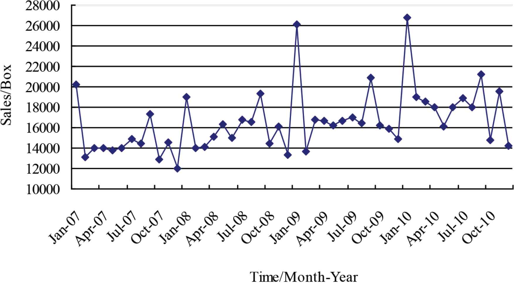
The original series of total monthly sales volume of cigarettes in G City, Guizhou, China from 2007 to 2010 was shown in Figure 1. The original data were from G City Branch, Guizhou Tobacco Company of China (see Table 1).
Original series.
| Time (month-year) | Original series (Box) | Moving average series (Box) | Ratio of original series to moving average series (%) | Seasonal factor (%) | Seasonally adjusted series (Box) | Smoothed trend-cycle series (Box) | Irregular (error) component |
|---|---|---|---|---|---|---|---|
| JAN-2007 | 20242.14 | — | — | 146.3 | 13839.430 | 14024.348 | 0.987 |
| FEB-2007 | 13116.56 | — | — | 91.3 | 14365.099 | 14122.436 | 1.017 |
| MAR-2007 | 13955.97 | — | — | 98.5 | 14162.779 | 14318.610 | 0.989 |
| APR-2007 | 14054.03 | — | — | 96.7 | 14534.791 | 14498.119 | 1.003 |
| MAY-2007 | 13811.13 | — | — | 93.7 | 14739.944 | 14628.354 | 1.008 |
| JUN-2007 | 14045.40 | — | — | 95.5 | 14708.150 | 14707.775 | 1.000 |
| JUL-2007 | 14883.09 | 14615.6077 | 101.8 | 100.7 | 14786.690 | 14750.661 | 1.002 |
| AUG-2007 | 14433.64 | 14516.1466 | 99.4 | 98.5 | 14657.462 | 14760.819 | 0.993 |
| SEP-2007 | 17377.90 | 14585.9138 | 119.1 | 116.4 | 14924.713 | 14852.390 | 1.005 |
| OCT-2007 | 12893.89 | 14601.8745 | 88.3 | 87.5 | 14744.025 | 14932.850 | 0.987 |
| NOV-2007 | 14535.67 | 14686.0441 | 99.0 | 95.0 | 15307.709 | 14826.872 | 1.032 |
| DEC-2007 | 12037.88 | 14896.2546 | 80.8 | 80.0 | 15041.271 | 14645.788 | 1.027 |
| JAN-2008 | 19048.61 | 14980.3642 | 127.2 | 146.3 | 13023.418 | 14375.738 | 0.906 |
| FEB-2008 | 13953.76 | 15134.6609 | 92.2 | 91.3 | 15281.998 | 14580.863 | 1.048 |
| MAR-2008 | 14147.50 | 15310.2532 | 92.4 | 98.5 | 14357.145 | 15027.746 | 0.955 |
| APR-2008 | 15064.06 | 15469.7871 | 97.4 | 96.7 | 15579.378 | 15707.082 | 0.992 |
| MAY-2008 | 16333.66 | 15598.9116 | 104.7 | 93.7 | 17432.113 | 16218.742 | 1.075 |
| JUN-2008 | 15054.72 | 15727.3979 | 95.7 | 95.5 | 15765.091 | 16420.960 | 0.960 |
| JUL-2008 | 16734.65 | 15838.1249 | 105.7 | 100.7 | 16626.259 | 16556.047 | 1.004 |
| AUG-2008 | 16540.75 | 16429.4141 | 100.7 | 98.5 | 16797.244 | 16562.548 | 1.014 |
| SEP-2008 | 19292.31 | 16409.1248 | 117.6 | 116.4 | 16568.869 | 16654.500 | 0.995 |
| OCT-2008 | 14443.38 | 16632.9389 | 86.8 | 87.5 | 16515.855 | 16671.881 | 0.991 |
| NOV-2008 | 16077.51 | 16768.1978 | 95.9 | 95.0 | 16931.437 | 16852.494 | 1.005 |
| DEC-2008 | 13366.60 | 16763.3228 | 79.7 | 80.0 | 16701.505 | 16805.299 | 0.994 |
| JAN-2009 | 26144.08 | 16901.4492 | 154.7 | 146.3 | 17874.548 | 16785.723 | 1.065 |
| FEB-2009 | 13710.29 | 16926.9555 | 81.0 | 91.3 | 15015.350 | 16546.676 | 0.907 |
| MAR-2009 | 16833.27 | 16918.0162 | 99.5 | 98.5 | 17082.714 | 16782.121 | 1.018 |
| APR-2009 | 16687.17 | 17051.2879 | 97.9 | 96.7 | 17258.007 | 17021.664 | 1.014 |
| MAY-2009 | 16275.16 | 17202.2155 | 94.6 | 93.7 | 17369.680 | 17293.307 | 1.004 |
| JUN-2009 | 16712.23 | 17187.1725 | 97.2 | 95.5 | 17500.818 | 17227.649 | 1.016 |
| JUL-2009 | 17040.72 | 17318.4606 | 98.4 | 100.7 | 16930.352 | 17164.595 | 0.986 |
| AUG-2009 | 16433.48 | 17374.2949 | 94.6 | 98.5 | 16688.309 | 17322.005 | 0.963 |
| SEP-2009 | 20891.57 | 17811.1228 | 117.3 | 116.4 | 17942.366 | 17561.015 | 1.022 |
| OCT-2009 | 16254.51 | 17956.3201 | 90.5 | 87.5 | 18586.865 | 17831.815 | 1.042 |
| NOV-2009 | 15896.99 | 18068.2965 | 88.0 | 95.0 | 16741.333 | 17890.310 | 0.936 |
| DEC-2009 | 14942.06 | 18050.0652 | 82.8 | 80.0 | 18670.030 | 18389.016 | 1.015 |
| JAN-2010 | 26814.09 | 18155.8828 | 147.7 | 146.3 | 18332.632 | 18826.967 | 0.974 |
| FEB-2010 | 18952.23 | 18306.9824 | 103.5 | 91.3 | 20756.256 | 19328.173 | 1.074 |
| MAR-2010 | 18575.64 | 18439.0649 | 100.7 | 98.5 | 18850.901 | 18981.047 | 0.993 |
| APR-2010 | 18030.89 | 18467.9041 | 97.6 | 96.7 | 18647.690 | 18611.562 | 1.002 |
| MAY-2010 | 16056.38 | 18346.4800 | 87.5 | 93.7 | 17136.192 | 18216.417 | 0.941 |
| JUN-2010 | 17982.04 | 18648.9966 | 96.4 | 95.5 | 18830.546 | 18352.578 | 1.026 |
| JUL-2010 | 18853.92 | 18587.4788 | 101.4 | 100.7 | 18731.804 | 18425.337 | 1.017 |
| AUG-2010 | 18018.47 | — | — | 98.5 | 18297.878 | 18287.517 | 1.001 |
| SEP-2010 | 21237.64 | — | — | 116.4 | 18239.582 | 18272.450 | 0.998 |
| OCT-2010 | 14797.42 | — | — | 87.5 | 16920.699 | 18268.385 | 0.926 |
| NOV-2010 | 19527.19 | — | — | 95.0 | 20564.345 | 18410.893 | 1.117 |
| DEC-2010 | 14203.85 | — | — | 80.0 | 17747.637 | 18482.148 | 0.960 |
Seasonal decomposition
It can be seen from Figure 1 that from 2007 to 2010, the original series shows the general characteristics of rising the bottom gradually and emerging two seasonal peaks in January and September every year. Therefore, it can be preliminarily judged that the total monthly sales volume of cigarettes in G City have the characteristics of double trend change of time series.
4.2. Test of the Holiday Effects
In this paper, the Spring Festival and National Day were selected as the holidays to investigate the holiday effects of cigarettes sales in G City. In order to facilitate comparison, the sample data were divided into two subgroups: the last month before the holiday (referred to as pre-holiday) and all other months (referred to as other). We used Excel software to make descriptive statistical analysis of sample data, and used Eviews7.2 software to do regression analysis of sample data.
The descriptive statistical analysis results of the original series were shown in Table 2. It can be seen from Table 1 that the pre-holiday average value is 21381.04 boxes, which is far higher than the other average value of 15631.69 boxes, reaching 1.3678 times. This preliminary shows that the cigarettes sales in G City have obvious pre-holiday effects. In addition, from the standard deviation point of view, the pre-holiday standard deviation is 3371.942 boxes, which is much higher than the other standard deviation of 1843.548 boxes, reflecting the greater pre-holiday volatility. Therefore, the follow-up needs to carry on the regression analysis to get the general conclusion.
| Subgroups | Average value/Box | Maximal value/Box | Minimal value/Box | Standard deviation/Box | Sample sizes | Multiple of average value |
|---|---|---|---|---|---|---|
| Pre-holiday | 21381.04 | 26814 | 17378 | 3371.942 | 8 | 1.3678 |
| Other | 15631.69 | 19527 | 12038 | 1843.548 | 40 | 1.0000 |
Multiple of average value, pre-holiday average value/other average value.
Descriptive statistical analysis results
Using Equation (1), a dummy variable model was constructed, and the pre-holiday effects of cigarettes sales in G City were then test. The test results were shown in Table 3.
| Variable | Coefficient | Std. Error | t-Statistic | Prob. |
|---|---|---|---|---|
| c | 15645.03 | 141.3023 | 110.7203 | 0.0000 |
|
|
5585.926 | 145.6055 | 38.36343 | 0.0000 |
Test results of the pre-holiday effects
Table 3 shows that the constant term c is 15645.03 and the regression coefficient α is 5585.926 in this model. The t-statistic of α is 38.36343, and the corresponding probability p-value is 0.0000, which shows that the regression coefficient α is significant at the 1% significance level. The goodness-of-fit (R2) of the model is 0.9696, and the adjusted goodness-of-fit (Adjusted R2) is 0.9690, which shows that the fitting effect of the model is good, and the independent variable can explain 96.96% difference of the dependent variable. The observed value of F-statistic is 1471.753, which is higher than the critical value (7.220) of F-test at the 1% significance level. Therefore, the hypothesis of zero is rejected, which shows that the linear relationship between dependent variable and independent variable is very significant, and a linear model can be established. The above results show that the cigarettes sales in G City have the statistically significant positive pre-holiday effects.
4.3. Seasonal Decomposition Results
According to Subsection 3.1, using the seasonal decomposition function provided by SPSS18.0 software, we selected “Multiplicative” model (system default option) in the “Model Type” option group, and selected “All points equal” in “Moving Average Weight”, thus, we can get the seasonal decomposition table, as shown in Table 1.
Based on the original series, according to the specified moving average method and period, we obtained the moving average series. Its purpose was to eliminate the seasonal factors in the original series and get the trend value of the original series. According to the multiplicative model, the trend factors were removed from the original series, and the ratio of original series to moving average series was then obtained. We averaged the ratio of the same month in each year to get 12 averages, and then divided the 12 averages by the total ratio average, therefore, the seasonal factor for each month can be obtained. After removing the seasonal component from the original series, we got the seasonally adjusted series, and then smooth it to get the smoothed trend-cycle series. Finally, the irregular (error) component was obtained by eliminating the cyclic fluctuation factors from the seasonally adjusted series [23]. The original series and seasonally adjusted series were shown in Figure 2.
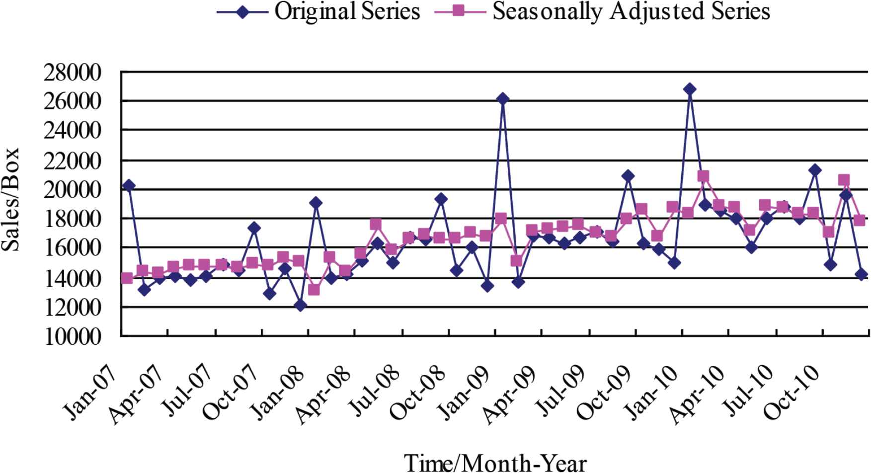
Original series and seasonally adjusted series.
In Figure 2, it can be seen that the original series shows the characteristics of fluctuating growth in annual cycle, and the seasonally adjusted series (i.e. the corrected monthly effects series) shows a steady growth trend in four years. The seasonal factor was shown in Figure 3.
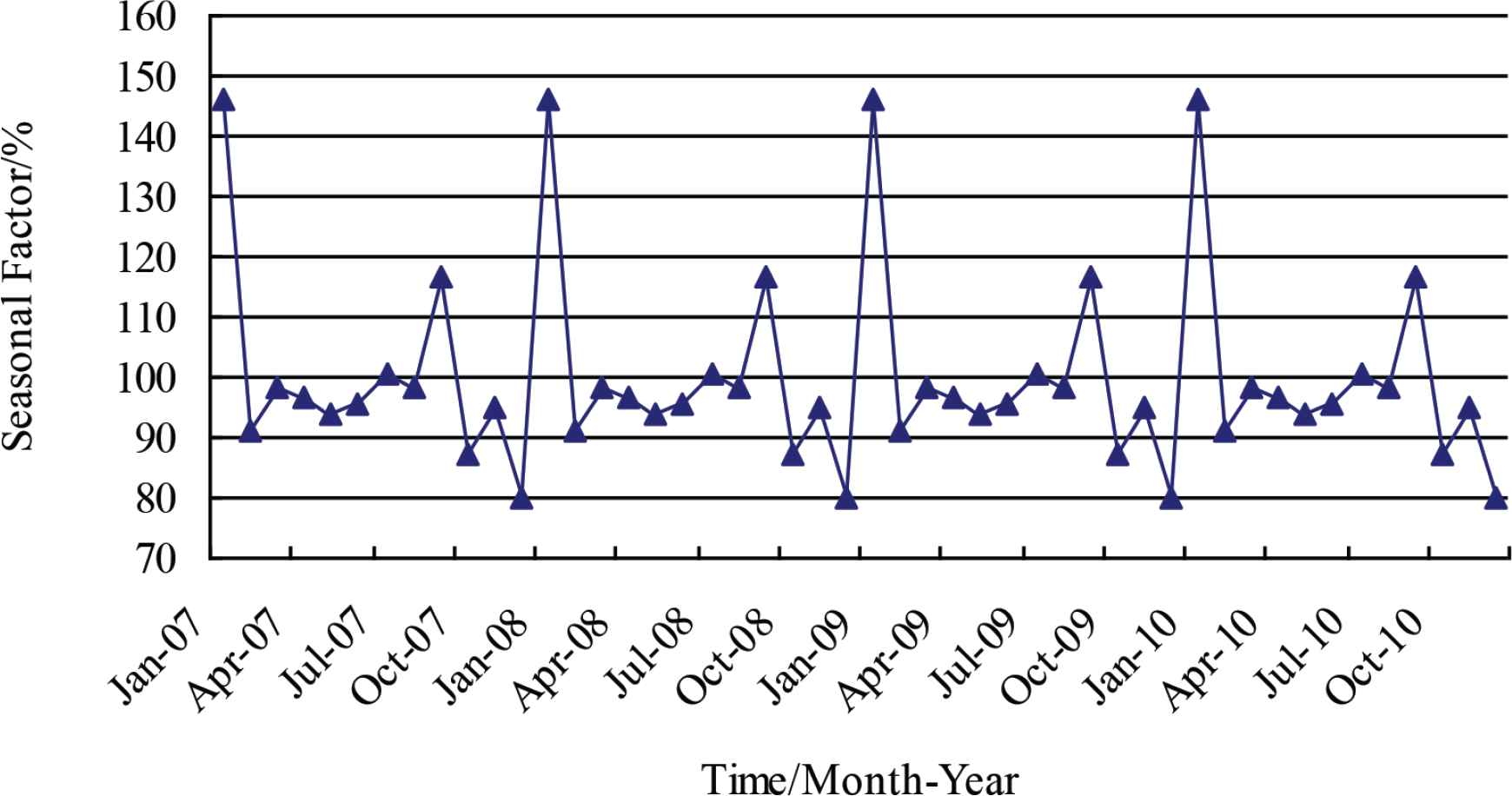
Seasonal factor.
In Figure 3, the seasonal factor fluctuates regularly in a 12-month period. It can be found that the sales volume of cigarettes in January and September are larger than that in other months. Figures 2 and 3 further verify the observations in Subsection 4.1.
4.4. Trend Forecast Results
According to Subsection 3.2, we used SPSS18.0 software to build the ARIMA(p, d, q) model and forecast the trend of the seasonally adjusted series.
- (1)
Stability test and processing. The Augmented Dickey–Fuller (ADF) test results shown that the seasonally adjusted series was a first-order stationary series, i.e. d = 1.
- (2)
Model recognition. Because the Partial Autocorrelation Function (PACF) graph and ACF graph of the stationary series were tailed, it can be determined that the stationary series was suitable for the ARMA model.
- (3)
Model order determination. The determining order method based on the optimal criterion function was used to determine the order of the model [24], i.e. we selected the group of orders minimizing the Akaike’s information criterion as the ideal order. Through the comparative test, the ARIMA(1, 1, 1) model was selected.
- (4)
Model test. Through observing the ADF test, ACF graph and PACF graph of the residual series of the ARIMA(1, 1, 1) model, it was confirmed that the residual series was the white noise series. Thus, the ARIMA(1, 1, 1) model was the best prediction model for the stationary series.
In the “Criteria” option group, we selected the “Nonseasonal ARIMA”, “None Transformation” and “Include constant in model”; selected the “Display forecasts” in the “Statistics” option group; set January to March 2011 as the forecast period in the “Selection” option group; and other items adopted the default options. The trend forecast results of the seasonally adjusted series were shown in Table 4.
| Months | 2011–01 | 2011–02 | 2011–03 |
|---|---|---|---|
| Forecast value/Box | 19426.1 | 19430.3 | 19547.5 |
| Upper limit value/Box | 21313.2 | 21319.1 | 21436.5 |
| Lower limit value/Box | 17539.0 | 17541.5 | 17658.6 |
The trend forecast results of the seasonally adjusted series
4.5. Sales Forecast Results
According to Subsection 3.3, refilling the trend forecast value in Table 4 with the seasonal factor in Table 1, i.e. the seasonal factor of the corresponding month was multiplied by the trend forecast value of the seasonally adjusted series, thus, the forecast results of the total monthly sales volume of cigarettes in G City from January to March 2011 were obtained, as shown in Table 5.
| Months | Actual value/Box | Forecast value/Box | Error/% | Upper limit value/Box | Error/% | Lower limit value/Box | Error/% |
|---|---|---|---|---|---|---|---|
| 2011–01 | 30756.98 | 28420.36 | −7.60 | 31181.21 | 1.38 | 25659.50 | −16.57 |
| 2011–02 | 18614.07 | 17739.86 | −4.70 | 19464.35 | 4.57 | 16015.38 | −13.96 |
| 2011–03 | 19315.71 | 19254.33 | −0.32 | 21114.98 | 9.32 | 17393.69 | −9.95 |
Error = (forecast value − actual value)/actual value.
The forecast results of the total monthly sales volume of cigarettes in G City from January to March 2011
Table 5 shows the relative error between the forecast value obtained by our model and the actual value of the total monthly sales volume of cigarettes in G City. The absolute average error after calculation is 4.20%, which shows that our model can better predict the change trend of the total monthly sales volume of cigarettes in G City, and can effectively simulate the seasonal, periodic and random characteristics of cigarettes sales. In addition, our model also gives the upper and lower limits of the forecast value, which provide a space for the empirical adjustment of the forecast value.
4.6. Comparative Analysis
In order to facilitate comparison, based on the original series, we also adopted respectively the nonseasonal ARIMA model, product seasonal ARIMA model [25] and seasonal exponential smoothing method - Winters multiplicative model to forecast the total monthly sales volume of cigarettes in G City from January to March 2011, the results were shown in Table 6. Where, the nonseasonal ARIMA (2, 1, 1) model and the product seasonal ARIMA(1, 1, 1)(1, 0 ,1) model were finally determined as the best prediction models for the stationary series after the modeling steps of stability test and processing, model recognition, model order determination and model test.
| Months | Actual value/Box | Nonseasonal ARIMA(2, 1, 1) | Product seasonal ARIMA(1, 1, 1) (1, 0, 1) | Winters multiplicative model | Our model | ||||
|---|---|---|---|---|---|---|---|---|---|
| Forecast value/Box | Error/% | Forecast value/Box | Error/% | Forecast value/Box | Error/% | Forecast value/Box | Error/% | ||
| 2011–01 | 30756.98 | 20631.91 | −32.92 | 26933.74 | −12.43 | 27552.18 | −10.42 | 28420.36 | −7.60 |
| 2011–02 | 18614.07 | 18583.61 | −0.16 | 18669.34 | 0.30 | 17834.00 | −4.19 | 17739.86 | −4.70 |
| 2011–03 | 19315.71 | 19305.21 | −0.05 | 19465.53 | 0.78 | 18958.20 | −1.85 | 19254.33 | −0.32 |
| Absolute Average Error/% | — | 11.05 | — | 4.30 | — | 5.49 | — | 4.20 | |
Error = (forecast value − actual value)/actual value.
Comparative analysis results
It can be seen from Table 6 that the absolute average error of our model is only 4.20%, which is lower than 5.49% of the Winters multiplicative model and 11.05% of the nonseasonal ARIMA(2, 1, 1) model, which is also slightly lower than 4.30% of the product seasonal ARIMA(1, 1, 1)(1, 0, 1) model. Especially in January 2011, when the seasonal fluctuation is prominent, the prediction error of our model is only −7.60%, which is significantly lower than the other three models. Which means that the prediction accuracy of our model is better, which shows good applicability in the double trend prediction and can meet the needs of practical application.
5. DISCUSSION
From the results and analysis of the previous section, we observed that our model was able to obtain the slightly higher prediction accuracy than the product seasonal ARIMA(1, 1, 1)(1, 0, 1) model [our method was 95.8%, and the product seasonal ARIMA(1, 1, 1)(1, 0, 1) model was 95.7%], and the higher prediction accuracy than the Winters multiplicative model and the nonseasonal ARIMA(2, 1, 1) model [the Winters multiplicative model was 94.51%, and the nonseasonal ARIMA(2, 1, 1) model was 88.95%].
Compared with the product seasonal ARIMA, Winters multiplicative model and the nonseasonal ARIMA model, our method can obtain the slightly higher or higher prediction accuracy. Since our model divides the sales forecasting into three stages. First, using the seasonal decomposition, the seasonal factor is separated from the original series, and the seasonally adjusted series is then obtained. Second, using the ARIMA model, a trend forecast to the seasonally adjusted series is further carried out. Finally, according to the multiplicative model, refilling the trend forecast value with the seasonal factor, thus, the final sales forecast results of the consumer goods with holiday effects can be obtained.
In addition, compared with literature [14], our model avoids the limitation of BP neural network in trend prediction. Compared with literature [15], our model overcomes the irrationality of hypothesis premise in trend prediction. Obviously, the advantage of our model is that it can give full play to the advantages of seasonal decomposition in dealing with seasonal change factor, and the advantages of ARIMA model in trend prediction at the same time. Therefore, our model has high prediction accuracy and low prediction risk in sales forecasting of the consumer goods with holiday effects. It should be noticed that the time span of the original series in this paper is from 2007 to 2010, and there are only 48 sample data, which may weaken the persuasiveness of the example analysis results. However, due to the trade secrets involved, the data problem cannot be solved temporarily.
6. CONCLUSION
There are so-called holiday effects in the sales of many consumer goods in reality, and their sales data have the characteristics of double trend change of time series, which leads to the decrease of prediction accuracy and the increase of prediction risk of quantitative prediction method. In view of this, by introducing the seasonal decomposition and ARIMA model, this paper proposed a sales forecasting model for the consumer goods with holiday effects. Taking the cigarettes sales in G City, Guizhou, China as an example, the feasibility and effectiveness of this new model was verified by the example analysis results. This paper provides a new method and idea for improving the sales forecasting accuracy of the consumer goods with holiday effects, which has high practical value.
The basic law of prediction is that the shorter the prediction period, the stronger the prediction ability of quantitative prediction method; the longer the prediction period, the weaker the prediction ability of quantitative prediction method. Therefore, in practical application, it is necessary to establish a sales forecasting system based on our model to make real-time dynamic sales forecast for the consumer goods with holiday effects.
It should be noticed that the seasonal decomposition artificially decomposes time series into four fixed components; however, its scientific nature needs to be further verified. In addition, since the information used in a single prediction method is limited, only one method is used to predict the same problem, the prediction accuracy is often not high, and the prediction risk is large [26]. Therefore, in order to improve the forecast effect, it is worth further study to establish a sales combination forecasting model for the consumer goods with holiday effects [27].
CONFLICTS OF INTEREST
The authors declare they have no conflicts of interest.
AUTHORS’ CONTRIBUTION
MZ contributed in conceived and designed the experiments. CY contributed in performed the experiments. XH contributed in analyzed the data. MZ and XH contributed in paper drafting and final revision.
ACKNOWLEDGMENTS
To the Regional Project of National Natural Science Foundation of China (71861003) and the Innovative Exploration and New Academic Seedlings Project of Guizhou University of Finance and Economics (Guizhou-Science Cooperation Platform Talents [2018] 5774-016) for their support.
REFERENCES
Cite this article
TY  - JOUR
AU  - Mu Zhang
AU  - Xiao-nan Huang
AU  - Chang-bing Yang
PY  - 2020
DA  - 2020/07/15
TI  - A Sales Forecasting Model for the Consumer Goods with Holiday Effects
JO  - Journal of Risk Analysis and Crisis Response
SP  - 69
EP  - 76
VL  - 10
IS  - 2
SN  - 2210-8505
UR  - https://doi.org/10.2991/jracr.k.200709.001
DO  - 10.2991/jracr.k.200709.001
ID  - Zhang2020
ER  -