
Deep High-Resolution Network for Low-Dose X-Ray CT Denoising
 , Dan Nguyen, Biling Wang, Steve Jiang*
- DOI
- 10.2991/jaims.d.210428.001How to use a DOI?
- Keywords
- Low-dose CT; Deep learning; Denoise
- Abstract
Low-dose computed tomography (LDCT) is clinically desirable because it reduces the radiation dose to patients. However, the quality of LDCT images is often suboptimal because of the inevitable strong quantum noise. Because of their unprecedented success in computer vision, deep learning (DL)-based techniques have been used for LDCT denoising. Despite DL models' promising ability to remove noise, researchers have observed that the resolution of DL-denoised images is compromised, which decreases their clinical value. To mitigate this problem, in this work, we developed a more effective denoiser by introducing a high-resolution network (HRNet). HRNet consists of multiple branches of subnetworks that extract multiscale features that are fused together later, which substantially enhances the quality of the generated features and improves denoising performance. Experimental results demonstrated that the introduced HRNet-based denoiser outperformed the benchmarked U-Net–based denoiser, as it provided superior image resolution preservation and comparable, if not better, noise suppression. Quantitative evaluation in terms of root-mean-squared errors (RMSEs)/structure similarity index (SSIM) showed that the HRNet-based denoiser improve these values from 113.80/0.550 (LDCT) to 55.24/0.745 (HRNet), which outperformed the 59.87/0.712 for the U-Net–based denoiser.
- Copyright
- © 2021 The Authors. Published by Atlantis Press B.V.
- Open Access
- This is an open access article distributed under the CC BY-NC 4.0 license (http://creativecommons.org/licenses/by-nc/4.0/).
1. INTRODUCTION
X-ray computed tomography (CT) is widely used in clinics to visualize the internal organs of patients for diagnostic purposes. However, the radiation dose involved in X-ray CT scans constitutes a potential health concern to the human body, since it may induce genetic, cancerous, and other diseases. Therefore, following the As Low As Reasonably Achievable (ALARA) principle is of the utmost importance in clinics when determining the radiation dose level of a CT scan. One of the dominant ways to reduce the dose level is to decrease the exposure level of each projection angle. However, lower exposure levels inevitably introduce stronger quantum noise into the CT image, which could make accurate diagnosis and organ contouring impossible, thereby decreasing the clinical value of these images. Thus, a denoising algorithm is essential for enhancing the image quality of low-dose CT (LDCT) images.
There has been a surge of research in this direction, which can be roughly divided into three categories: projection domain–based denoising [1,2], image domain–based denoising [3,4], and regularized iterative reconstruction [5–12]. Because it is convenient to access the CT images directly from the picture archive and communication system (PACS), image domain–based denoising algorithms are becoming increasingly popular. In this work, we devote our efforts to this last category, as we seek to enhance the image quality of LDCT.
Inspired by the unprecedented successes of convolutional neural network (CNN)-based deep learning (DL) techniques [13] in various image processing [14–18] and recognition [19–23] tasks, the medical community has widely adopted them to denoise CT images [24–31], achieving state-of-the-art denoising performance. For instance, Chen et al. devised a deep CNN consisting of several repeating convolutional modules that learns a mapping from LDCT images to normal-dose CT (NDCT) images [25]. To facilitate a more efficient information flow and to compensate the potential spatial resolution loss, they further proposed a new architecture that uses the well-known residual learning scheme, called residual encoder–decoder (RED) [25], and attained better denoising performance. This improvement in performance may be attributed to the more advanced architecture design. Indeed, it is well-recognized that neural network architecture is one of the dominant factors that affects an algorithm's performance, since it directly affects the qualities of the features, which are an abstract representation of the image. Moreover, the development history of CNN-based DL techniques over the past decade can be organized in terms of the evolution of the associated architectures: the original AlexNet [19] contained several convolutional layers and fully connected layers, then the VGG [32] network substantially increased the network's depth; the inception network [33] considered multiscale structures, then the well-known ResNet [22] proposed a residual connection to facilitate the information propagation; and most recently, the feature pyramid network (FPN) [34] fused the low- and high-level features. Many other architecture variants have been developed, such as SENet [35], DenseNet [36], and ResNeXt [37]. As network architectures have evolved, the associated algorithms' performance has also improved substantially, as in the case of the top-5 error rate of the well-known ImageNet 1K dataset being reduced from 20.91% (AlexNet) to 5.47% (ResNeXt).1
The goal of our LDCT image denoising task is to suppress the noise effectively while preserving the resolution as much as possible, since noise and resolution are two important, but combating, metrics for evaluating CT image quality. High-level features are key to effectively suppressing noise by aggregating information from a large receptive field, while low-level features are essential for preserving good resolution. Therefore, extracting high-quality low- and high-level features and effectively fusing them will be extremely important when designing CNN architectures for LDCT image denoising. Toward this technical line, U-Net [38] might be one of the most well-known architectures, which add a skip connection to facilitate the fusion of the low- and the high-level features. Despite its great success in various tasks and datasets, researchers have found that applying the U-Net architecture to the LDCT denoising task still leads to significant resolution loss, thus decreasing the clinical value of the denoised CT images. Therefore, there is still room to further enhance the image quality of the denoised CT image by employing a more advanced network architecture that can extract and fuse the low- and high-level features more effectively.
In the field of natural image processing and analysis, Sun et al. [39] and Wang et al. [40] proposed a high-resolution network (HRNet)-based representation learning method that attained state-of-the-art performance across various computer vision tasks, such as human pose estimation, image classification, object detection, and segmentation. Specifically, HRNet uses multiple branches to extract multiscale features, which are then fused together internally. This architecture design can ensure a highly efficient combination of low- and high-level features during the forward propagation process and thus produce a high-quality feature for the downstream task.
To the best of our knowledge, this architecture has not been applied to denoising tasks. We feel that HRNet is highly suitable for medical image denoising tasks where high resolution is desirable to preserve the fidelity of anatomical structures. Given this, in this work, we have introduced HRNet into the medical image processing field and verified its superior denoising performance for LDCT images. We hope this newly introduced architecture will also help other researchers in the medical imaging field to boost performance on this task.
2. METHODS AND MATERIALS
2.1. Methods
Let us first mathematically formulate our problem. Given an LDCT image
From the perspective of DL, problem (1) can be regarded as an image-to-image translation problem that can be solved by learning a CNN
In practice, one can never access a real clean image that contains no noise, since quantum noise is inevitable. Therefore, the clean image in the training dataset is usually replaced with an NDCT image
For completeness, we illustrate the architecture of the HRNet in Figure 1. There are four different branches that extract the features from different scales. The starting feature of each scale is calculated by applying a stride-two convolutional layer to the feature of the previous scale. All features from the different scales are processed in a stage-by-stage fashion. Each stage contains two convolutional layers, as indicated by the solid arrows in Figure 1. Before proceeding to the next stage, the features from different scales are fused together. In this work, this fusion process is based on the feature summation. Specifically, if the size of the previous feature is larger than that of the current feature (such as fusing the features from branch 1 into the features from branch 3), one or more stride-two convolutional layers are used to downsample the previous feature so that it has the same size as the current feature. For example, if the previous feature has a size of
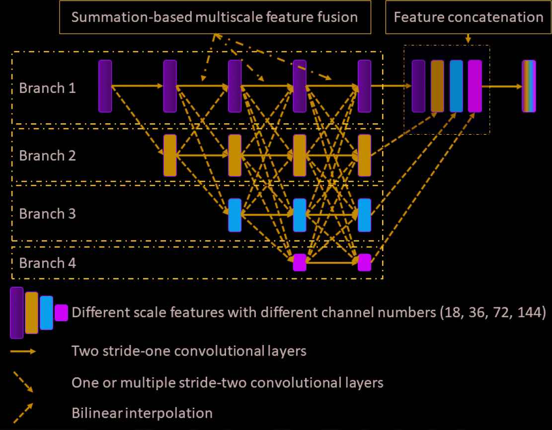
Illustration of the HRNet architecture. Four different branches extract the features from different scales. During the forward propagation, the features from different scales are fused together gradually. To enable the fusion process, indicated by the dashed line connections, the previous features are first downsampled or upsampled, depending on the relative size of the features, such that the summation-based feature fusion is valid. Finally, all the features from the different scales are upsampled to the original scale, if necessary, and concatenated together, resulting in the final features. A predictor is attached as the last layer to output the denoised image. All convolutional layers consist of three operators: convolution, instance normalization, and rectified nonlinear unit. The final predictor consists of two operators: convolution and rectified nonlinear unit.
In this work, all convolutional layers except the predictor consist of three operators: a convolution operator, an instance normalization [41] operator, and the rectified nonlinear unit (ReLU). The predictor consists of the convolution operator and the ReLU. The channel number for the features in same scale is the same. Specifically, all the convolution operators in the 1st/2nd/3rd/4th branch have the same input and output channel numbers, which are 18/36/72/144, respectively. We use stride-two convolutional layers (stacked if necessary) to conduct the downsampling operation. In details, if we downsample a feature from branch i to a feature in branch j, we will use ceil
2.2. Materials
2.2.1. Training and validation datasets
In this work, we used the publicly released American Association of Physicists in Medicine (AAPM) Low-Dose CT Grand Challenge dataset [42], which consists of contrast-enhanced abdominal CT examinations, for the model training (https://www.aapm.org/grandchallenge/lowdosect/). Specifically, NDCT projections were first acquired according to the routine clinical protocols at Mayo Clinic, which uses the automated exposure control and automated tube potential selection strategies so that the referenced tube potential is 120 kV and the quality referenced effective exposure is 200 mAs. Then, Poisson noise was inserted into the projection data to reach a noise level that corresponded to
The official training dataset comprises data from ten patients. For qualitative evaluation, we randomly split these into eight and two patients to serve as the training and validation datasets, respectively. All the data involved in this work are in 2D slices. In total, there were 4800 and 1136 2D CT slice images in the training and validation datasets, respectively.
For showcase purposes, we chose four representative slices in the validation dataset to demonstrate and compare the denoising performance. The first slice was used to check the denoising performance for the abdominal site, which is the dominant site of the training dataset. The second slice corresponds to the liver, which is one of the most important human organs in the abdominal site. The third slice selected was in the lung region, which was partially covered during the CT scan. The fourth slice contains a radiologist-confirmed low-contrast lesion.
2.2.2. Testing dataset
We used patient's data from the testing dataset of the challenge to verify the model's performance. Specifically, we first rebinned the raw helical-scanned projection data into fan-beam projection data with a slice thickness of
2.2.3. Training details
The input and target images were the LDCT and NDCT images, respectively. In detail, we first normalized both images by dividing by 2000 so that most of the image intensities fell within the range of 0–1. Note that the pixel values of the original CT images are CT values that were shifted by 1000 HU.
To enlarge the dataset, we have conducted extensive data augmentations. Specifically, given an image of size
We used the Adam [43] optimizer to minimize the cost function (2), with hyperparameters
2.2.4. Comparison studies
For comparison, we also implemented a baseline network architecture: U-Net.
To be specific, in the encoder part, the initial output channel number in the input layer is 32. Continuous stride-two convolutional layers are applied to extract images' high-level features. The channel number is doubled per each downsampling resulting from the stride-two convolutional operators until a feature number of 512 is reached. There are nine layers in the encoder part, which leads to a bottleneck feature with a size of
All other training details for the U-Net were the same as for the HRNet introduced above.
2.2.5. Evaluation metrics
In this work, we evaluated the models' performance quantitatively in terms of the root-mean-square error (RMSE) and the structure similarity (SSIM) [44]. The RMSE is defined as
The SSIM is defined as
We quantified the detectability of lesions via the contrast-to-noise ratio (CNR). The CNR is defined as follows:
2.2.6. Noise analysis
As mentioned above, the model was trained with paired LDCT-NDCT images, where both the input LDCT and the target NDCT images were contaminated by noise. More specifically, the target NDCT image contained realistic quantum noise (denoted as target noise hereafter), while the input LDCT image contained both the target noise inherited from the NDCT image and the added simulated noise (denoted as added noise hereafter). We decided that it would be interesting and valuable to analyze whether the trained denoiser can remove both the target noise and the added noise.
We first defined the difference between the input LDCT and the output denoised image as removed noise. We used the cosine correlations between the removed noise and the added noise or the target noise to characterize the composition of the removed noise. More specifically, since the target noise is coupled with the underlying clean image, and there may be a certain number of structures in the removed noise, we calculated the cosine correlations based on the high- frequency components, where the majority is the noise. In this work, the high- frequency components are defined as those frequencies in the ranges of
As a showcase, we used all the slices from one patient in the validation dataset to analyze the noise correlations.
3. RESULTS
Figure 2 presents the denoised results for a slice in the validation dataset corresponding to the abdominal site. It is obvious that both denoisers effectively suppressed the noise, as shown in Figure 2(b) and 2(c). Compared to the NDCT image in Figure 2(d), the U-Net–based denoiser produced an image with much inferior resolution. The HRNet-based denoiser introduced here produced an image (Figure 2[c]) with much better resolution than the U-Net–based denoiser, but with slightly inferior resolution to the NDCT image. These phenomena can be clearly observed from the zoomed-in views displayed in the second row of Figure 2. In addition, the noise level of the image associated with the HRNet-based denoiser is much lower than that of the NDCT image. Another interesting finding is that using the U-Net–based denoiser led to strong artifacts around the boundary of the bone, as indicated by the red arrows in the third row of Figure 2. By contrast, the HRNet-based denoiser faithfully restored the underlying structures around that region.
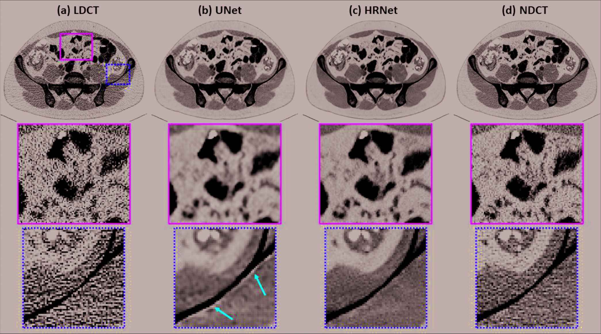
Denoised results for the slice selected from the abdominal site. (a) LDCT, (b) U-Net, (c) HRNet, and (d) NDCT. Images in the second and third rows are the zoomed-in views for the contents in the first row, corresponding to the regions of interest indicated by the solid green box and the dotted yellow box, respectively. Display window: [−160, 240] HU.
Figure 3 demonstrates the denoised results for the liver organ. The strong noise in the LDCT image overwhelms the fine vessels in the liver. Both denoisers suppressed the noise effectively. Observing the zoomed-in view in the second row of Figure 3 reveals that the HRNet-based denoiser produced an image with more details, thus suggesting higher resolution, than the U-Net–based denoiser. Moreover, the noise in the image associated with the HRNet-based denoiser is weaker than in the image from the U-Net–based denoiser, which indicates the HRNet's stronger denoising ability. The red arrows indicate that some of the vessels in the image from the HRNet-based denoiser can be more easily distinguished than even those in the NDCT image, which also suffers from the quantum noise.
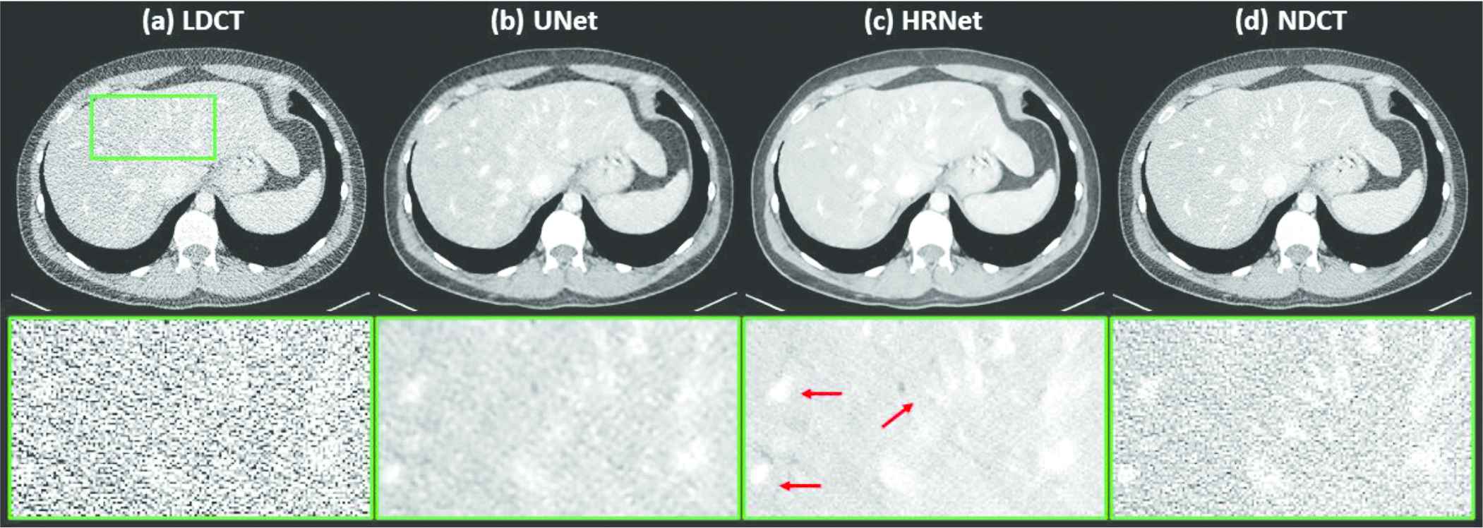
Denoised results for the slice corresponding to the liver organ. (a) LDCT, (b) U-Net, (c) HRNet, and (d) NDCT. Images in the second row are the zoomed-in views for the contents in the first row, corresponding to the region of interest indicated by the solid green box. Display window: [−160, 240] HU.
Figure 4 depicts the denoised results for the lung slice. In this case, both the LDCT and the NDCT images clearly show the locations and shapes of the lung nodules. Processing the LDCT with the U-Net–based denoiser substantially decreased the resolution even though the noise was effectively removed. The image generated by the HRNet-based denoiser exhibits much weaker noise than, but slightly inferior, if not comparable, resolution to the LDCT image. Indeed, as the red arrows in Figure 4 indicate, these small lung nodules have clearer structures than in the LDCT image, which is contaminated by strong quantum noise.
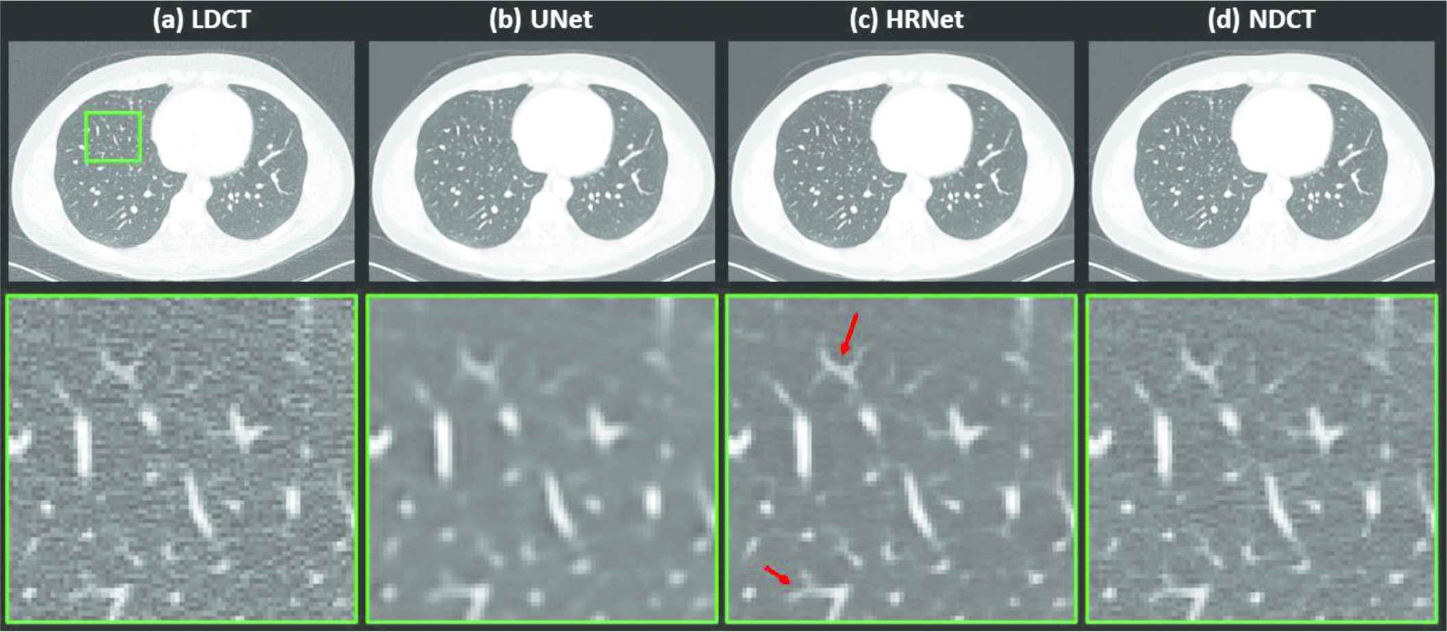
Denoised results for the slice corresponding to the lung region. (a) LDCT, (b) U-Net, (c) HRNet, and (d) NDCT. Images in the second row are the zoomed-in views for the contents in the first row, corresponding to the region of interest indicated by the solid green box. Display window: [−160, 240] HU.
Figure 5 compares different denoising results by using the slice that contains a low-contrast lesion, indicated by the solid green box. Not surprisingly, it is hard to distinguish this lesion from the surrounding normal tissues on the noisy LDCT image. Using the denoisers greatly alleviates this challenge, as shown by the images in Figure 5(b) and 5(c). Further inspection of both denoised images reveals that the HRNet-based denoiser yielded an image with a much more natural noise texture. This can be clearly seen in the zoomed-in views in the second row of Figure 5. For quantitative comparison, we also calculated the CNRs of this low-contrast lesion on different images, with results of 0.32 (LDCT), 2.45 (U-Net), 2.70 (HRNet), and 0.90 (NDCT); this further verifies the superior denoising performance of the introduced HRNet-based denoiser.
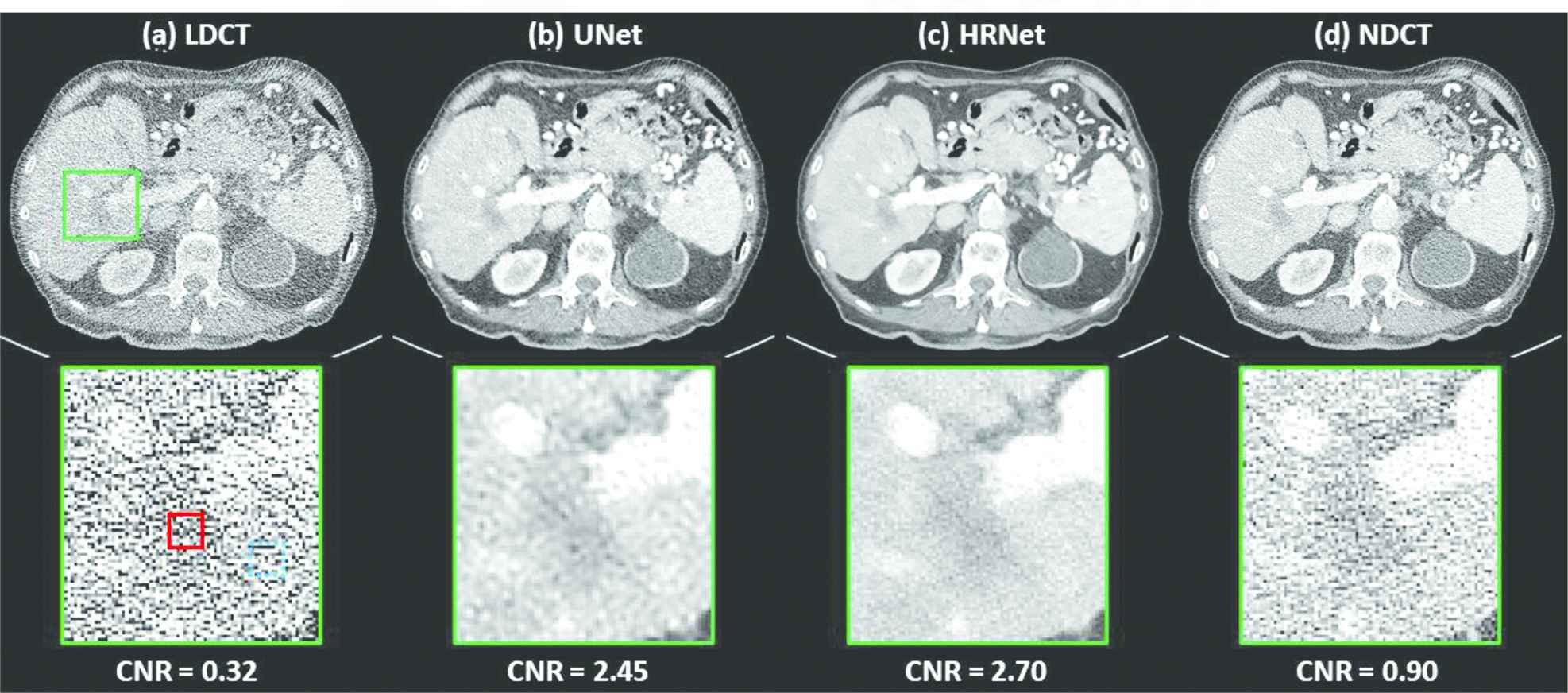
Denoised results for the slice containing a low-contrast lesion, as indicated by the solid green box. (a) LDCT, (b) U-Net, (c) HRNet, and (d) NDCT. Images in the second row are the zoomed-in views of the low-contrast lesion. The red solid box and the blue dotted box indicate the foreground and background contents, respectively, used for the CNR calculation, and the associated results are shown below. Display window: [−160, 240] HU.
To further quantify the performance of both denoisers, we calculated the RMSE and SSIM values for each showcase in Figures 2–5 with their reference NDCT images, as listed in Table 1. We can see that both denoisers dramatically reduced the RMSE values, but the HRNet-based denoiser yielded a greater improvement than the U-Net–based denoiser. Similar findings can also be observed from the SSIM-based metrics. For a more comprehensive comparison, we calculated and plotted the RMSE and SSIM values for all the slices in the validation dataset (Figure 6). This plot shows that the introduced HRNet-based denoiser outperformed the U-Net–based denoiser in almost every evaluated slice, even though both denoisers substantially enhanced the image quality. For an overall quantitative comparison, we also computed the averaged RMSE and SSIM values for the entire validation dataset. As tabulated in Table 1, the RMSE decreased from 113.80 HU (LDCT) to 59.87 HU when applying the U-Net–based denoiser, and it decreased further to 55.24 HU with the HRNet-based denoiser. Again, the SSIM values also validate the image quality enhancement, as they increased from 0.550 (LDCT) to 0.712 (U-Net) and 0.745 (HRNet).
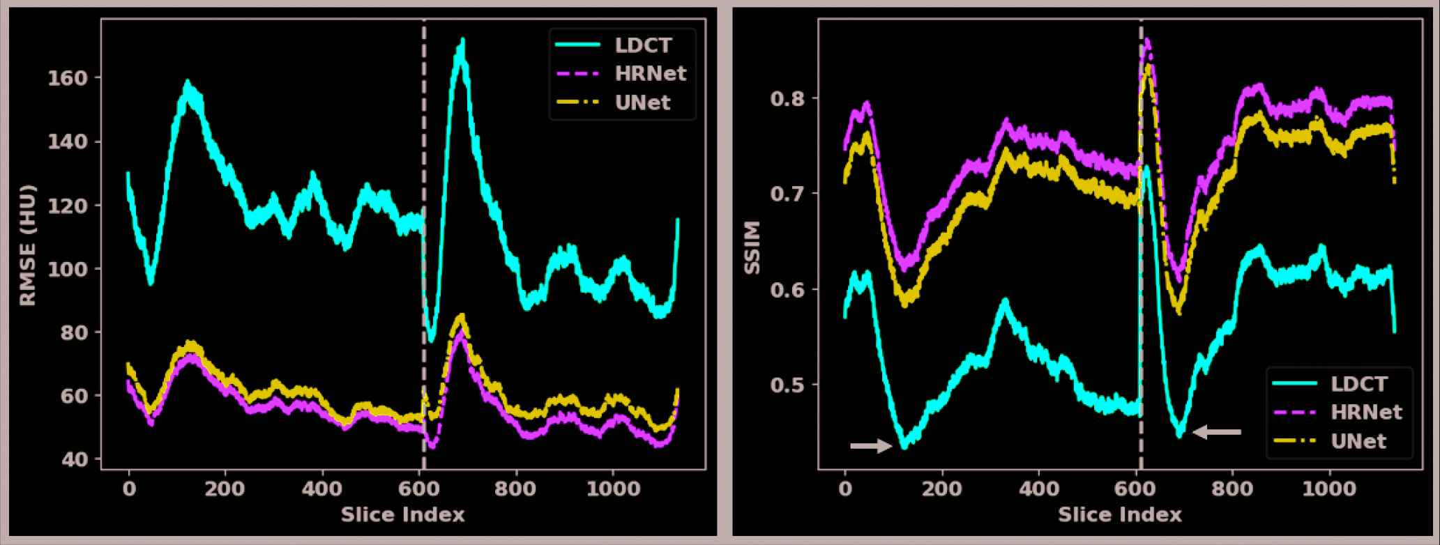
Quantitative results for each slice in the validation dataset. The x-axes are the slice index and the y-axes are the RMSE (left figure) and the SSIM (right figure). The solid red, dashed green, and dotted dash blue curves pertain to the LDCT, the HRNet method, and the U-Net method, respectively. The slices of the two patients in the validation dataset are separated by the dashed black vertical line.
| Figure 2 | Figure 3 | Figure 4 | Figure 5 | Dataset | ||
|---|---|---|---|---|---|---|
| RMSE (HU) | LDCT | 115.49 | 124.67 | 120.90 | 164.52 | 113.80 |
| U-Net | 61.08 | 63.84 | 66.65 | 82.32 | 59.87 | |
| HRNet | 56.10 | 60.55 | 61.01 | 76.94 | 55.24 | |
| SSIM | LDCT | 0.571 | 0.516 | 0.588 | 0.451 | 0.550 |
| U-Net | 0.734 | 0.666 | 0.727 | 0.584 | 0.712 | |
| HRNet | 0.766 | 0.702 | 0.761 | 0.620 | 0.745 | |
To further investigate the denoising performance boundary of the introduced HRNet-based denoiser, in Figure 7, we demonstrate two worst cases in terms of the lowest SSIM values for the two patient cases in the validation dataset. It clearly reveals that the proposed HRNet-based denoiser still outperforms the U-Net–based denoiser, with better noise suppression and superior details preservation ability. This can be also verified from the quantitative metrics as tabulated in Table 2.
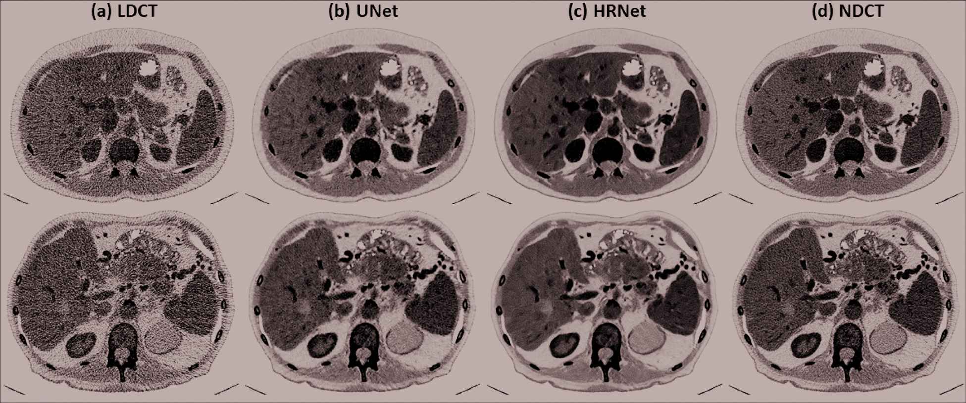
Denoised results for the two slices that exhibits the lowest SSIM values in the two validation patients. (a) LDCT, (b) U-Net, (c) HRNet, and (d) NDCT. The images in the first and the second rows correspond to the slices indicated by the left and the right arrows in Figure 6 (SSIM subfigure). Display window: [−160, 240] HU.
| Figure 7 | Top Row | Bottom Row | |
|---|---|---|---|
| RMSE (HU) | LDCT | 153.61 | 164.67 |
| U-Net | 74.49 | 82.87 | |
| HRNet | 70.71 | 77.60 | |
| SSIM | LDCT | 0.441 | 0.454 |
| U-Net | 0.692 | 0.584 | |
| HRNet | 0.629 | 0.620 | |
Quantitative results in terms of RMSE and SSIM for the two worst showcases in Figure 7 from the two patient cases in the validation dataset. The RMSE has a unit of HU.
The denoising results for a slice in the testing dataset are shown in Figure 8. We can see that the HRNet-based denoiser delivered an image with sharper edges and a comparable, if not weaker, noise level than the U-Net–based denoiser.

Denoised results for the slice in the testing dataset. (a) LDCT, (b) U-Net, and (c) HRNet. Display window: [−160, 240] HU.
The noise analysis is shown in Figure 9. We can observe that the difference image (Figure 9[b]) between the input and the denoised images contains almost exclusively noise, which suggests that the introduced HRNet-based denoiser preserved structural details very well. The corresponding Fourier domain depicted in Figure 9(c) suggests that the noise is dominated by both the low- and the high-frequency components, while the middle-frequency noise has been effectively removed. After we masked out the low-frequency part (Figure 9[f]) and inversely transformed back to the image domain (Figure 9[e]), the noise contained only the high-frequency component, which can be clearly observed by comparing Figure 9(b) and 9(e). Since the low-frequency component is excluded, the noise power in Figure 9(e) is lower than in Figure 9(b). The cosine correlations among the different noise components are plotted in Figure 9(d). We can see that the target noise and the extra added noise are almost orthogonal, with a cosine correlation of around −0.08, which is close to zero. The correlation is around 0.9 between the removed noise and the extra added noise and around 0.3 between the removed noise and the target noise. These two values indicate that most of the removed noise comes from the extra added noise, though the denoiser also removes some noise from the target image. The projection length from the removed noise to the extra added noise is 78.46%, and the projection length from the removed noise to the target noise is 61.31%. After we subtract the projected noise from the removed noise, the remaining noise has an energy of 11.37% of all the removed noise.
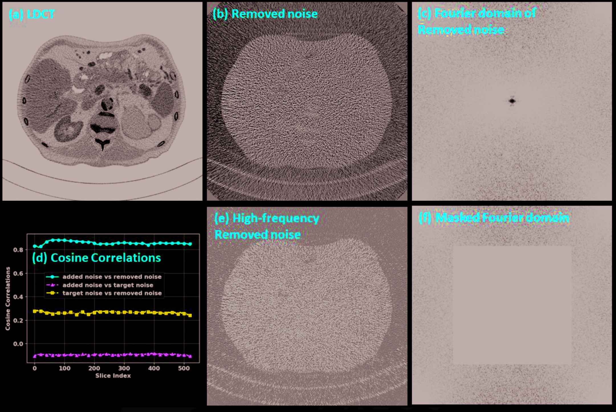
Noise analysis. (a) LDCT, (b) noise removed by the HRNet-based denoiser, (c) Fourier domain of the removed noise, (d) cosine correlations among the added noise, the removed noise and the target noise, (e) the high-frequency components of the removed noise, and (f) the masked Fourier domain. The display window is [−160, 240] HU for image (a), [−50, 50] HU for images (b) and (e), and [104, 105] HU for images (c) and (f).
4. DISCUSSIONS AND CONCLUSIONS
The goal of any CT denoiser is to suppress the noise as much as possible while preserving anatomical details as well as possible. DL–based denoisers have proven very effective at suppressing noise by automatically extracting image features, thus achieving state-of-the-art denoising performance. However, the feature quality highly depends on the model architecture. For the denoising task, both the low- and the high-level features are important. The former is important for preserving details, while the latter is essential for effectively suppressing noise by using context information on a large scale. The encoder–decoder architecture is efficient for high-level feature extraction, but it lacks low-level information. The U-Net can improve the low-level feature quality to some extent by using skip connections, but still cannot provide a high low-level feature quality that can be used to faithfully restore the fine details. This deficiency can be clearly observed from Figure 2 where there exist strong dark artifacts around the boundary of the bone regarding the U-Net–based denoising result, as indicated by the red arrows. This extracted low-quality low-level feature probably also explain why the U-Net–based denoiser leads to oversmoothed structures despite it can suppress the noise effectively. By contrast, the introduced HRNet generated both low- and high-level features of high quality by using different branches to extract the features from different levels, then fusing the different level features together. Consequently, our experimental results verified the superiority of this architecture design and showed that HRNet can effectively remove noise while preserving the fine anatomical structures very well.
For some cases, the results from the HRNet were even better than the NDCT, such as for the low-contrast lesion detection task (Figure 5). This might be because we removed not only the added simulated noise but also the noise inherited from the target NDCT image. The noise analysis above supports our hypothesis, as it shows that the HRNet-based denoiser removed 61.31% of the target noise from the NDCT image. Nonetheless, we are not claiming that the HRNet-based denoiser can deliver an image whose quality surpasses that of NDCT. Actually, when visualizing high-contrast details that are robust to the noise but sensitive to the resolution, such as the lung nodules shown in Figure 4, the structures associated with the HRNet are slightly oversmoothed compared to the NDCT.
It is well known that data-driven DL models may suffer from the problem of model generalizability when there is a distribution gap between the training and the testing environments. In this work, the models were tested only on simulated datasets whose data distributions are similar to the training dataset, if one ignores the potential differences caused by different reconstruction parameters. More realistic testing datasets are required to evaluate the model's performance further before it can be translated to the clinic.
In summary, in this work, we introduced an HRNet-based denoiser to enhance the quality of LDCT images. Because it extracts both low- and high-level features of high quality, the HRNet can deliver an enhanced image with effectively suppressed noise and well preserved details. Compared to the U-Net–based denoiser, the HRNet can produce images with higher resolution. Quantitative experiments showed that the introduced HRNet-based denoiser can improve the RMSE/SSIM values from 113.80/59.87 (LDCT) to 55.24/0.745, and it outperformed the U-Net–based denoiser, whose values are 59.87/0.712.
DATA AVAILABILITY
The data used in this paper can be publicly accessed from the official website of the AAPM Low-Dose CT Challenge (https://www.aapm.org/grandchallenge/lowdosect/).
CONFLICTS OF INTEREST
The authors declare they have no conflicts of interest.
AUTHORS' CONTRIBUTIONS
Steve Jiang: Initiated the project; Ti Bai, Biling Wang, Dan Nguyen and Steve Jiang: Designed the experiments; Ti Bai: Performed the model training; Biling Wang: Conducted the data collection and the data analysis: Ti Bai: Wrote the paper; Steve Jiang: Edited the paper.
ACKNOWLEDGMENTS
We would like to thank Varian Medical Systems Inc. for supporting this study and Dr. Jonathan Feinberg for editing the manuscript. We also would like to thank Dr. Ge Wang from Rensselaer Polytechnic Institute for his constructive discussions and comments.
Footnotes
These data come from the model zoo provided by the official implementations of PyTorch. See https://pytorch.org/docs/stable/torchvision/models.html for more details.
REFERENCES
Cite this article
TY  - JOUR
AU  - Ti Bai
AU  - Dan Nguyen
AU  - Biling Wang
AU  - Steve Jiang
PY  - 2021
DA  - 2021/05/03
TI  - Deep High-Resolution Network for Low-Dose X-Ray CT Denoising
JO  - Journal of Artificial Intelligence for Medical Sciences
SP  - 33
EP  - 43
VL  - 2
IS  - 1-2
SN  - 2666-1470
UR  - https://doi.org/10.2991/jaims.d.210428.001
DO  - 10.2991/jaims.d.210428.001
ID  - Bai2021
ER  -