
Multimedia Analysis and Fusion via Wasserstein Barycenter
- DOI
- 10.2991/ijndc.k.200217.001How to use a DOI?
- Keywords
- Multimedia analysis; Wasserstein Barycenter; fusion
- Abstract
Optimal transport distance, otherwise known as Wasserstein distance, recently has attracted attention in music signal processing and machine learning as powerful discrepancy measures for probability distributions. In this paper, we propose an ensemble approach with Wasserstein distance to integrate various music transcription methods and combine different music classification models so as to achieve a more robust solution. The main idea is to model the ensemble as a problem of Wasserstein Barycenter, where our two experimental results show that our ensemble approach outperforms existing methods to a significant extent. Our proposal offers a new visual angle on the application of Wasserstein distance through music transcription and music classification in multimedia analysis and fusion tasks.
- Copyright
- © 2020 The Authors. Published by Atlantis Press SARL.
- Open Access
- This is an open access article distributed under the CC BY-NC 4.0 license (http://creativecommons.org/licenses/by-nc/4.0/).
1. INTRODUCTION
Many multimedia analysis algorithms rely on probability distributions that characterize audio or image features as generally high dimensions. For example, music analysis methods, such as automatic music transcription (AMT) [1] and music classification [2], in these applications, having sufficient similarity (or equivalent difference) between distributions becomes crucial. The classical distance or difference of probability density includes Kullback Leibler divergence, Kolmogorov distance, Bhattacharyya distance (also known as Hellinger distance), etc. Recently, the framework of optimal transportation and Wasserstein distance [3] are also called earth mover’s distance (EMD) [4], which has aroused great interest in computer vision [5], machine learning [6] and data fusion. Wasserstein distance calculates the best warped starter to map the measure μ to the second ν for a given input probability. Optimality corresponds to a loss function that measures the predicted value of the displacement in the warped starter. Generally, considering the accumulation of μ and ν, Wasserstein distance calculates the definition of the displacement of every particle from traces of its mass to the displacement of μ to ν.
In this paper, the applications of Wasserstein Barycenter [7] algorithm in music transcription and classification are discussed. The first application described in this paper is music transcription. In this study, we use non-negative matrix factorization (NMF) as the method of converting audio signal to musical instrument digital interface (MIDI) format and Wasserstein Barycenter as the algorithm of data fusion. The second is music classification, first we used jSymbolic software to extract the key features, and then input these features into our traditional machine learning model including eXtreme gradient boosting (XGB), back propagation neural network (BPNN), support vector machine (SVM). Finally, we propose Wasserstein Barycenter as the ensemble method of these models. Wasserstein distance, also known as EMD, is used to measure the distance between two distributions. Compared with Kullback Leibler (KL) and Jenson-Shannon (JS)–divergence, Wasserstein distance has the advantage that even if the support sets of two distributions do not overlap or overlap very little, it can still reflect the distance between the two distributions.
The remaining sections are organized as follows: In Section 2, we first review some of the theorems in the literature and mainly present the theorems of Wasserstein Barycenter, methodology of music transcription and model of music classification. Section 3 conducts experiment result of music transcription and music classification. Section 4 introduces the evaluation methods and the comparison of different models. In Section 5, we summarize our work and present future research directions in the field.
2. RELATED WORK
Materials show that the Wasserstein distance presents a useful methodology for quantifying geometric differences between the different distributions. In particular, they are mostly applied as variables in content-based image retrieval [8], modeling and visualization of image intensity value [9–12], estimated average probability metrics (i.e. Barycenter of gravity) [13,14], cancer detection [15,16], super resolution [17] and other applications. Recent advances in variation minimization [18,19], particle approximation [20], multi-scale schemes [21,22], and entropy regularization [5,6,23], transmission metrics can be effectively utilized to pattern recognition, machine learning and signal processing issues. Moreover, Wang et al. [10] describes a theory for computing the transport distance (expressed as linear optimal transport) between N image data sets requiring N minimized distance problems. Rabin et al. [14] and Bonneel et al. [23] proposes the truth that these problems are easy to solve for distribution of one-dimension, and introduces a change in the local distance defined as the Sliced Wasserstein distance. Finally, recent work [24–26] shows that the transmission frames can be treated as a reversible signal conversion framework allowing signal classes to be more linearly separated for various pattern recognition and machine learning tasks.
Due to the benefits of using the above transport distances and Wasserstein distance, and taking into account the flexibility and strength of Wasserstein Barycenter [7] algorithm, ensemble methods using Wasserstein Barycenter in dealing with data fusion have been described with applications in music transcription and music classification.
Various research groups of polyphonic pitch detection used different techniques for music transcriptions. Yeh et al. [27] presented a cross pitch estimation algorithm based on the score function of a pitch candidate set. Nam et al. [28] posed a transcription approach which uses deep belief networks to calculate a mid-level time-pitch representation. Duan et al. [29] and Emiya et al. [30] proposed a model of spectral peak, non-peak region and the residual noise via Maximum Likelihood (ML) methods. More recently, Peeling and Godsill [31] raised a F0 estimation function and an inhomogeneous Poisson in the frequency domain. In spectrogram factorization-based multi-pitch detection, resulting in harmonic and inharmonic NMF, Vincent et al. [32] merged harmonic constraints in the NMF model. Bertin et al. [33] presented a Bayesian model based on NMF, and each pitch in harmonic positions is treated as a model of Gaussian components. Fuentes et al. [34] modeled each note as a weighted amount of narrowband log spectrum, and switched to log frequency with the convoluted PLCA algorithm. Abdallah and Plumbley [35] combined machine learning and dictionary learning via non-negative sparse coding.
Since the emergence of the Internet, music classification has been a widely studied field. Researchers around the world have put a lot of energy into the field of music classification. Although researchers have proposed different algorithms from different perspectives, most of them rely on excellent and well-designed designs and the construction of appropriate classifiers for music data. Traditional music classification methods are based on supervised machine learning [36]. They used k-Nearest Neighbor (KNN) and Gaussian Mixture model. The above methods as well as Mel-frequency Cepstral coefficients were used for noisy classification. Lee et al. [37] introduced a multiclass SVM approach that translated multiple classification problems into a single optimization problem rather than breaking it down into multiple binary classification problems. There are many favorable properties of Wasserstein distance, which are recorded in theories [3] and practice [38]. With the recent success of Deep Neural Networks (DNN), a number of studies apply these techniques to speech and other forms of audio data. Hussain and Haque [39] developed SwishNet— a fast CNN for audio data classification and segmentation. AzarNet, a DNN was created by Azar et al. [40] to recognize classical music. Liu et al. [41] fully exploited of low-level information in the audio from spectrograms to develop a new CNN algorithm. Nasrullah and Zhao [42] reviewed the classification method of artists under this framework and conducted an empirical study on the impact of introducing time structure into feature representation. Under the comprehensive conditions, they applied the convolutional recursive neural network to the music artist recognition data set and established the classification architecture.
Based on the recent works on EMD [4] and Wasserstein Barycenter [7], we propose a converged method and have concrete theoretical and practical advantages in music transcription and classification. We derive mathematical results that enable Wasserstein Barycenter ensemble to be applied in music transcription and music classification. Finally, we prove through experiments that Wasserstein Barycenter ensemble outperform the commonly used models such as SVM, XGB and BPNN.
3. METHODOLOGY
Our idea of music signal processing ensemble is inspired by the recent study on EMD and Wasserstein Barycenter in the area of machine learning. Here, we introduce their formal definitions first. And then we propose music classification models with compared classifiers.
3.1. Music Transcription with Earth Mover’s Distance
Let X = {x1, x2, ..., xn1} and Y = {y1, y2, ..., yn1} be two sets of weighted points in Rd with non-negative weights αi and βj for each αi ∈X and βj ∈Y respectively, and WX and WY be their corresponding total weights. The EMD [4,43] between X and Y is
Roughly speaking, EMD is an example of the least cost and maximum flow problem in the Euclidean space Rd. Therefore, the problem of computing EMD can be solved by linear programming [44]. In addition, several faster algorithms have been proposed by using the techniques developed in computational geometry [43,45,46]. Following EMD, we have the definition of Wasserstein Barycenter.
3.2. Music Classification with Compared Classifiers
3.2.1. Multiclass SVM
Support vector machine is a useful technique for data classification. Even though it is considered that neural networks are easier to use than this; however, sometimes unsatisfactory results are obtained. A classification task usually involves with training and testing data which consist of some data instances. Each instance in the training set contains one target values and several attributes. The goal of SVM is to produce a model which predicts target value of data instances in the testing set which are given only the attributes.
Classification in SVM is an example of Supervised Learning. Known labels help indicate whether the system is performing in a right way or not. This information points to a desired response, validating the accuracy of the system, or be used to help the system learn to act correctly. A step in SVM classification involves identification as which are intimately connected to the known classes. This is called feature selection or feature extraction. Feature selection and SVM classification together have a use even when prediction of unknown samples is not necessary. They can be used to identify key sets which are involved in whatever processes distinguish the classes.
Computing the SVM classifier amounts to minimizing an expression of the form
Minimizing (2) can be rewritten as a constrained optimization problem with a differentiable objective function in the following way.
For each i ∈ {1, ..., n}, we introduce a variable ζi = max(0, 1 − yi(w · xi − b)). Note that ζi is the smallest non-negative number satisfying yi(w · xi − b) ≥ 1 − ζi.
Thus we can rewrite the optimization problem as to minimize
By solving for the Lagrangian dual of the above problem, one obtains the simplified problem, which is to maximize
Moreover, ci = 0 exactly when
The offset b can be recovered by finding an
Sub-gradient decent algorithms for the SVM work directly with the expression
Note that f is a convex function of
Coordinate descent algorithms for the SVM work from the dual problem, which is to maximize
One of the major strengths of SVM is that the training is relatively easy. No local optimal, unlike in neural networks. It scales relatively well to high dimensional data and the trade-off between classifier complexity and error can be controlled explicitly. The weakness includes the need for a good kernel function.
3.2.2. Multilevel Wasserstein means
For any given subset Θ ⊂ Rd, let P(Θ) denote the space of Borel probability measures on Θ. The Wasserstein space of order r ∈ [1, ∞) of probability measures on Θ is defined as
• Wasserstein distances
For any elements G and G′ in Pr(Θ) where r ≥ 1, the Wasserstein distance of order r between G and G′ is defined as:
By a recursion of concepts, we can speak of measures of measures, and define a suitable distance metric on this abstract space: the space of Borel measures on Pr(Θ), to be denoted by Pr(Pr(Θ)). This is also a Polish space (that is, complete and separable metric space) as Pr(Θ) is a Polish space. It will be endowed with a Wasserstein metric of order r that is induced by a metric Wr on Pr(Θ) as follows: for any D, D′ ∈ Pr(Pr(Θ)),
• Wasserstein barycenter
Next, we present a brief overview of Wasserstein barycenter problem. Given probability measures (P1, P2, ..., PN ∈ P2(Θ)), for N ≥ 1, their Wasserstein barycenter PN,λ is such that
Efficient algorithms for finding local solutions of the Wasserstein barycenter problem over Ok(Θ) for some k ≥ 1 have been studied recently in Cuturi and Doucet [48].
3.2.3. eXtreme gradient boosting
eXtreme gradient boosting, proposed by Dr. Chen in 2016, is a large-scale machine learning method for tree boosting and the optimization of gradient boosting decision tree (GBDT). As a lot of researches have mentioned, GBDT is an ensemble learning algorithm, which aims to achieve accurate classifications by combining a number of iterative computation of weak classifiers (such as decision trees). However, unlike GBDT, XGB can take advantage of multi-threaded parallel computing by using central processing unit (CPU) automatically to shorten the process of iteration. Besides, additional regularization terms help decrease the complexity of the model.
In Supervised Learning, there are objective function as well as predictive function. In XGB, objective function in Equation (10) consists of training loss L(ϕ) which measures whether model is fit on training data and regularization Ω(ϕ) which measures complexity of model. If there is no regularization or regularization parameter is zero, the model returns to the traditional gradient tree boosting.
When it comes to L(ϕ):
Then the corresponding objective function is:
And the model after t times iteration:
The formula of second-order Taylor expansion is:
In this formula,
When it comes to Ω( f ):
In Equation (17), q(xi) structure function, which describes the structure of a decision tree ω is the weight of the leaves on the tree. Equation (18) describes the complexity of a tree. γ is a coefficient of leaf nodes, taking pre-processing to prune leaves while optimizing the objective function. λ is another coefficient to prevent the model from over-fitting.
Define Pi = {i|q(xi) = j} as the sample set for each leaf j. Then the objective function can be simplified as:
When structures of trees q are known, this equation has solutions:
Blessed with traits mentioned above, XGB has the following advantages compared to traditional methods:
- (i)
Avoiding over-fitting. According to Biasvariance trade-off, the regularization term simplifies the model. Simpler models tends to have smaller variance, thus avoiding overfitting as well as improving accuracy of the solution.
- (ii)
Supporting for parallelism. Before training, XGB sorts the data in advance, and saves it as a block structure. When splitting nodes, we can calculate the greatest gain of each feature with multi-threading by using this block structure.
- (iii)
Flexibility. XGB supports user-defined objective function and evaluation function as long as the objective function is second-order derivable.
- (iv)
Built-in cross validation. XGB allows cross validation in each round of iterations. Therefore, the optimal number of iterations can be easily obtained.
- (v)
Process of missing feature values. For a sample with missing feature values, XGB can automatically learn its splitting direction.
3.2.4. Back propagation neural network
Back propagation neural network is a multi-layer feedforward neural network trained by error back propagation learning algorithm. It was firstly coined by Rumelhart and McClelland in 1986. Blessed with strong ability of nonlinear mapping, generalization and fault tolerance, it has become one of the most widely used neural network models. The core of BPNN mainly includes two parts: the forward propagation of signals as well as the reverse propagation of errors. In the former, input signals as input cells activate the cells of hidden layer and transfer information to them with weights. The hidden layer also acts on the output layer in this way, thus finally getting the output results. If those results are not fit on the expected output results, it turns to the latter process. The output layer error will be back-propagated layer by layer. The weights of the network are adjusted at the same time to make the output of the forward propagation process closer to the ideal output.
• Forward propagation
First, we need to introduce activation functions. It helps to solve complex non-linear problems. The widely used activation function is the sigmoid function:
In input layer, the input and output of the ith cell are the same. And the number of input cells is n1.
In hidden layer, the input and output of the ith cell are as follows. And the number of input cells is n2.
In output layer, the input and output of the kth cell are as follows:
• Back propagation
We define the expected output as Ô and the number of the output cells is n3. After training, the total error is:
According to the chain rule, we can adjust the weights.
Similarly, other weights can also be adjusted in this way.
4. EXPERIMENT
4.1. Experiment of Music Transcription
4.1.1. Database and data preprocessing
In this section, we start to describe training data and experimental settings, and then conduct the state-of-the-art method to merge different transcription results. In this experiment, we use anaconda3 and python3.5 to perform the transcription, and sklearn toolbox to deal with data; while adopted pycharm to merge the data of different transcription results.
In data preparation period, the instrumental sound records in studio were described as dry source; however, most of scenes were not ideal. For a large amount of ground noise would be added to dry source during recording due to the sound card device or background. What’s more, some instrumental sound was recorded in different scenes and added different noises. We chose three classical music pieces by Bach, Mozart and Beethoven and preprocessed them with filter noise, distortion noise, reverb noise and dynamic noise.
4.1.2. Experimental settings
In this paper, we first propose a method based on NMF. Then we employed a fresh and simple Time-frequency representation, using the effectiveness of spectral features when highlighting the start time of notes. In addition, we adopted the NMF model to input the proposed features. In our system, we used different audio signals recorded in different scenes with a sample rate of 48 kHz. We split the frame with a hamming window of 8192 samples and a jump size of 1764 samples. The 16,384-point DFT was calculated on every frame via double zero padding. Smoothing the spectrum through a median filter covered 100 ms. The algorithm is updated and iterated 50 times. Each row of the transcription results showed: onset time, offset time, notations of MIDI are as follows in Figure 1.
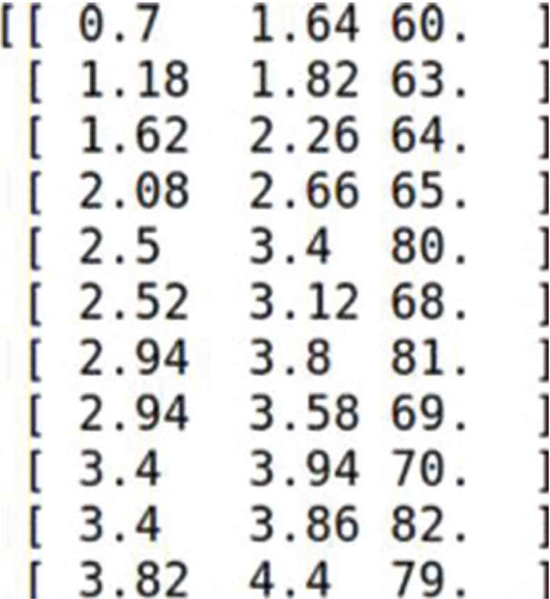
The transcription result.
4.2. Experiment of Music Classification
4.2.1. Database and data preprocessing
As for data sets, we selected classical music from five composers. They are Haydn, Mozart, Beethoven, Bach and Schubert. We get 200 pieces of music from each composer, a total of 1000 pieces. We use 90% of each composer’s data as a training set and the remaining 10% is used as testing set. Music pieces are all in MIDI format.
4.2.2. Experimental settings
In this experiment, we use python 3, an interpretative scripting language. We mainly use sklearn toolbox to deal with data, which is simple but efficient tools for data mining and data analysis. It is not only accessible to beginners but also reusable in various contexts. Matplotlib toolbox is used to draw the receiver operating characteristic curve (ROC curve).
4.2.3. Features extraction
In this paper, we use jSymbolic as an open-source platform for extracting features from symbolic music. These features can serve as inputs to machine learning algorithms, or they can be analyzed statistically to derive musicological insights. jSymbolic implements 246 unique features, comprising 1497 different values, making it by far the most extensive symbolic feature extractor to date. These features are designed to be applicable to a diverse range of music, and may be extracted from both symbolic music files as a whole and from windowed subsets of them.
Features extracted with jSymbolic can be roughly divided into eight categories, which are: range, repeated notes, vertical perfect fourths, rhythmic variability, parallel motion, vertical tritones, chord duration, number of pitches. And the following is a brief introduction of some of them.
- •
Pitch Statistics: How common are various pitches and pitch classes relative to one another? How are they distributed and how much do they vary?
- •
Chords and Vertical Intervals: What vertical intervals are present? What types of chords do they represent? What kinds of harmonic movement are present?
- •
Rhythm: Information associated with note attacks, durations and rests, measured in ways that are both dependent and independent of tempo. Information on rhythmic variability, including rubato, and meter.
5. RESULTS AND COMPARISON
5.1. Comparison of Music Transcription
5.1.1. Ensemble and comparison
First, we examined data sets in four scenes (adding filter noise, distortion noise, reverb noise and dynamic noise) under which we could get reasonable clusters. Then, we used the Wasserstein Barycenter algorithm as our ensemble method to obtain results. For example, we put forward the transcription data with reverb noises before ensemble. While, we generated the 10 transcription data adding with different reverb noises and then merged them through Wasserstein means algorithm.
We show that ensemble method is more robust than single transcription method in four scenes through Proportional Transportation Distance (PTD). The experimental results are evaluated objectively by using PTD described above. The PTD is computed by first dividing each point’s weight by the total weight of its point set, and then the EMD of resulting point sets is calculated [52]. According to the EMD and PTD method, we present notation as sets of weighted points. The weight represents note duration. Each note stands for a point distributed in the x and y coordinates, representing the start time and pitch, respectively. We use the Euclidean distance as the ground distance.
5.1.2. Evaluation
We conducted the evaluation by calculating precision (P = Ntp/(Ntp + Nfp)), recall (R = Ntp/(Ntp + Nfn)), F-measure (F = 2PR/(P + R)) and accuracy (A = Ntp/(Ntp + Nfp + Nfn)), where Ntp, Nfp and Nfn are the numbers of true positives, false positives and false negatives respectively. If the pitch is correct and its starting time is within 50 ms of the ground truth, we computed the notes as true positives [53].
The results are shown in Table 1. First of all, we averaged precision, recall, F-measure and accuracy of unmerged data from three composers in four scenes. Then, we compared the values of them in four scenes with those of merged data. It can be seen that the ensemble method is better than single transcription method in four scenes and the rates of precision, recall, F-measure and accuracy are obviously higher than those of unmerged data. It has increased nearly two times in F-measure and accuracy and 1.5 times in precision and recall.
| Precision | Recall | F-measure | Accuracy | |
|---|---|---|---|---|
| Filter | 0.4321 | 0.6667 | 0.3766 | 0.3232 |
| Reverb | 0.4405 | 0.6829 | 0.3841 | 0.3927 |
| Dynamic | 0.4272 | 0.6977 | 0.3385 | 0.3431 |
| Distortion | 0.4137 | 0.6914 | 0.3278 | 0.3703 |
| Ensemble | 0.6241 | 0.9231 | 0.7371 | 0.6642 |
Performance comparison on the real data set
5.2. Comparison of Music Classification
5.2.1. Ensemble and comparison
In this section, we combine different classifiers including SVM, XGB and BPNN to the ensemble classifier called Wasserstein Barycenter ensemble, which is based on Wasserstein Barycenter described above. Such an ensemble scheme which combines the prediction powers of different classifiers makes the overall system more robust. In our case, each classifier outputs a prediction probability for each of the classification labels. Hence averaging the predicted probabilities from the different classifiers would be a straightforward way to do ensemble learning.
The methodologies described in Section 3.2 that introduce different models of classification and the Wasserstein Barycenter algorithm, which makes sense to combine the models via ensemble. The performance of SVM, XGB, BPNN and WB ensemble is shown in Figure 2. ROC curve of BPNN has more twists and turns, compared with that of XGB, and ROC curve of WB ensemble is more smooth than that of SVM. The ROC curve for the WB ensemble model is above that of SVM, XGB and BPNN as illustrated in Figure 2. As shown in Table 2, this WB ensemble is beneficial and is observed to outperform the all individual classifiers.
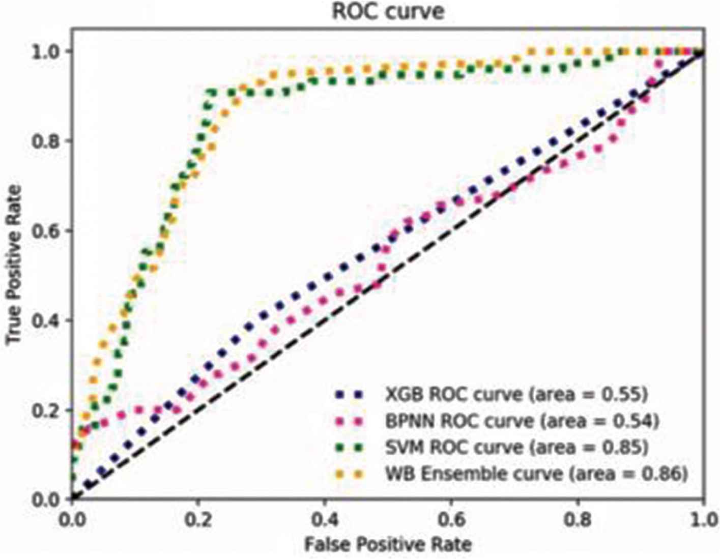
ROC curves for the best performing models and their ensemble.
| Classifiers | Accuracy | Precision | Recall | F-measure | AUC |
|---|---|---|---|---|---|
| SVM | 0.46 | 0.43 | 0.45 | 0.4 | 0.85 |
| XGB | 0.63 | 0.31 | 0.4 | 0.35 | 0.55 |
| BPNN | 0.43 | 0.18 | 0.26 | 0.22 | 0.54 |
| WB ensemble | 0.65 | 0.44 | 0.47 | 0.44 | 0.86 |
Performance comparison on classifiers and their ensemble
5.2.2. Evaluation
In order to evaluate the performance of the models described in Section 3.2, we compute precision, recall, F-measure, accuracy and area under curve (AUC) as the evaluation metrics of these classifiers. Experiment results can be seen from Table 2. The best performance in terms of all metrics is observed for ensemble model based on Wasserstein Barycenter. As we can see, WB ensemble achieves a classification effect better than other classifiers in each evaluation metric. There is no notable difference in AUC between XGB and BPNN, with 0.55 and 0.54 representatively. In contrast, SVM and WB ensemble reach to 0.85 and 0.86, higher than XGB and BPNN. In terms of accuracy, XGB has achieved 63%, nearly the same accuracy with WB ensemble, which has reached to 65%. However, in other evaluation metrics, SVM obviously performs better than XGB and BPNN.
Among the models that use manually crafted features, the one with the least performance is the BPNN model. This is expected since BPNN mainly deal with the classification of big data while our datasets are very small. SVMs outperform random forests in terms of AUC. However, the XGB version of the gradient boosting algorithm performs the best among the feature engineered methods with the relatively high accuracy.
6. CONCLUSION
In this paper we showed that Wasserstein Barycenter is effective in multiple scenes ensemble in music transcription and multiple classifiers ensemble in music classification. Here, we proposed two applications of Wasserstein Barycenter ensemble. For music transcription, in different scenes and pieces of music, we presented their effectiveness in ensemble results, as well as in improving the robustness and accuracy of music transcriptions. In addition, for music classification, we compare the performance of single classifiers and ensemble model for music style classification with different composers. Then, we also conduct an objective evaluation to compare diverse scenes and diverse models through measuring the differences between music signal data and the ground truth scores. Finally, we drew a conclusion that our crowdsourcing method is very useful in improving the robustness and accuracy of music signal processing results.
CONFLICTS OF INTEREST
The authors declare they have no conflicts of interest.
FUNDING
This research was supported by
REFERENCES
Cite this article
TY  - JOUR
AU  - Cong Jin
AU  - Junhao Wang
AU  - Jin Wei
AU  - Lifeng Tan
AU  - Shouxun Liu
AU  - Wei Zhao
AU  - Shan Liu
AU  - Xin Lv
PY  - 2020
DA  - 2020/02/26
TI  - Multimedia Analysis and Fusion via Wasserstein Barycenter
JO  - International Journal of Networked and Distributed Computing
SP  - 58
EP  - 66
VL  - 8
IS  - 2
SN  - 2211-7946
UR  - https://doi.org/10.2991/ijndc.k.200217.001
DO  - 10.2991/ijndc.k.200217.001
ID  - Jin2020
ER  -