
A Driving Behavior Awareness Model based on a Dynamic Bayesian Network and Distributed Genetic Algorithm
Guotao Xie and Hongbo Gao contributed equally to this work
- DOI
- 10.2991/ijcis.11.1.35How to use a DOI?
- Keywords
- Automated Vehicle; Advanced Driver Assistance System; Driving Behavior Awareness; Dynamic Bayesian Network; Distributed Genetic Algorithm
- Abstract
It is necessary for automated vehicles (AVs) and advanced driver assistance systems (ADASs) to have a better understanding of the traffic environment including driving behaviors. This study aims to build a driving behavior awareness (DBA) model that can infer driving behaviors such as lane change. In this study, a dynamic Bayesian network DBA model is proposed, which includes three layers, namely, the observation, hidden and behavior layer. To enhance the performance of the DBA model, the network structure is optimized by employing a distributed genetic algorithm (GA). Using naturalistic driving data in Beijing, the comparison between the optimized model and other non-optimized models such as the hidden Markov model (HMM) and HMM with a mixture of Gaussian outputs (GM-HMM) indicates that the optimized model could estimate driving behaviors earlier and more accurately.
- Copyright
- © 2018, the Authors. Published by Atlantis Press.
- Open Access
- This is an open access article under the CC BY-NC license (http://creativecommons.org/licences/by-nc/4.0/).
1. Introduction
Automated vehicles (AVs) and advanced driver assistance systems (ADASs) have received extensive research interest because they show great potential for use in more efficient, safer, and cleaner transportation systems1. It is evident that developments in this field will increase in both quality and importance over time2. For AV and ADAS to understand the environment, particularly in complex traffic scenarios, situation awareness (SA) is indispensable. The work of SA is to perceive environmental elements, comprehend their meaning, and project their status for the near future3,4. Driving behavior awareness (DBA) is a kind of SA for the automated vehicle and ADAS to have the comprehension of driving behaviors such as vehicle cut-in, stop or go, and turning left or right at the intersection5.
DBA helps AVs and ADASs to have a better understanding of the traffic environment in an abstract aspect. Moreover, DBA such as vehicle cut-in awareness plays a crucial role in driving strategies. Taking the cut-in scenario as an example, when a vehicle in the adjacent lane cuts in, the AV has to be aware of the adjacent vehicles cut-in behavior with the aim of changing its strategies, such as slowing down, and changing from a car-following model to a lane-changing model. Otherwise, the AV may suddenly brake or cause a serious traffic accident. In addition, in the interaction scenario, DBA could contribute to AVs deciding whether to slow down or go straight. Moreover, DBA models play a significant position in current ADASs such as lane-keeping as well as lane-departure systems. With the development of Vehicle-to-Vehicle (V2V) and Vehicle-to-Infrastructure (V2I) communication technologies, vehicles could share information including control information such as steering angle, and braking pedal signals. This information helps a vehicle estimate the other vehicles driving behavior more accurately.
To date, DBA models have been researched extensively.
Machine learning is one of the common methods to gain experience and knowledge from data6–12. The Bayesian network approach was used in this problem, and Dagli et al. developed a cutting-in vehicle recognition model with sensors available for adaptive cruise control (ACC) systems7. Bender et al. presented an unsupervised learning method for converting naturalistic driving data into high-level behaviors8. Dogan et al. compared the behavior estimating performance of machine learning methods such as the support vector machine, recurrent neural network, and feed forward neural network11. Nilsson et al. formulated simple logic rules for intention recognition of highway maneuvers12. These methods did not consider the influences of the historic information.
Further, game-theoretical approaches were used to model driving behaviors such as lane-changing and merging behavior. Talebpour et al. presented a model to understand and predict lane-changing behavior based on a game-theoretical approach that endogenously accounts for the flow of information in a connected vehicular environment13. Liu et al. modeled vehicle interactions during a merging process under an enhanced game-theoretical framework14. The testing results showed that this framework could predict a vehicles actions with relatively high accuracy. The combination of interaction-aware intention estimation with maneuver-based motion prediction on the basis of supervised learning is proposed and the motion intention is modeled by the game theoretical approach15.
Moreover, Markov models were employed and researched extensively to estimate driving behaviors16. Song et al. developed the intention-aware decision making model for an uncontrolled intersection. In their study, two layered HMMs were used to model driving intentions17. Using continues hidden Markov model (CHMM), driver intention of changing lane could be estimated in an early stage18. In this paper, the steering wheel angle, steering wheel angle velocity and lateral acceleration were used as optimal observation signals. Gadepally et al. built a framework for estimating driving decisions at an intersection19. Their research used HMMs to infer driving decisions from filtered continuous observations near the intersection. Furthermore, dynamic Bayesian network was widely used in driving behavior estimation because of its ability to deal with time sequential information. Ontann et al. mentioned the framework of the dynamic Bayesian network for learning from observations20. Li et al. developed a driving intention inference model by considering past driving behavior using dynamic Bayesian network theory21. In their study, the auto-regression HMM was used to consider past behavior to infer driving intention. Moreover, Lefvre et al. described a probabilistic framework to estimate a drivers intended maneuvers, which was applied in interaction scenarios22. Nonetheless, most of the research was based on a specific network structure.
The objective of this study is to build a DBA model based on a dynamic Bayesian network23 and distributed GA, with the aim to obtain experience and inference knowledge from naturalistic driving data. This DBA model includes three layers namely the observation layer, hidden layer and behavior layer. The network is shown in Fig. 1. The structure of the DBA network is difficult to optimize even using the GA. In this study, distributed GA is used, which has received considerable attention as it could reduce the execution time and improve the searching performance for the global optimal result, particularly in large complex system40. Furthermore, the evaluation indexes of DBA were proposed by considering the recognition start and succeed delay time (introduced in Section 4) for estimating driving behavior.
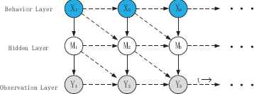
A DBA network composing the observation layer, hidden layer and behavior layer. Y represents the observation parameters, X indicates the behavior parameters and M is the hidden parameter. t reflects the time flow.
2. Dynamic Bayesian Network based DBA Model
In this section, a DBA model is proposed on the basis of the dynamic Bayesian theory, which includes three layers, namely the observation, hidden, and behavior layers. This section includes a brief review of DBA modeling and parameter learning for a specific network structure.
2.1. DBA modeling
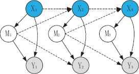
Based on the dynamic Bayesian theory, the DBA model is defined as a directed acyclic graph (DAG), composing a prior Bayesian network B1 and a two-slice temporal Bayes net B→ according to the first-order Markov assumption. This is shown in Fig. 2. The nodes in the network, representing variables such as driving behaviors, are connected by arcs and parameters expressed as conditional probabilistic distributions.
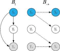
Dynamic-Bayesian-network-based DBA model.
In the network, the DBA is modeled as a stochastic process using continuous observations. A set of random variables in the networks are defined in terms of Zt = (Xt, Mt, Yt), where Xt represents the driving behavior at time t, Mt represents the hidden parameters in the network and Yt represents the observation parameters at time t. Moreover, B1 is a Bayesian network, which defines the prior P(Zt), and B→ defines the P(Zt|Zt−1) by means of DAG. This definition can be expressed as follows:
The network in this study is defined by unrolling the two-time slice temporal Bayesian network until T time slices are obtained. The resulting joint distribution is expressed as follows:
In this study, if the node Z and its parent nodes Pa(Z) are all discrete variables, then
If the node is continuous and its parent nodes are discrete variables, then the condition distribution could be expressed as follows:
Finally, if the node is continuous and its parent nodes are continuous variables, then
For example, in the structure of HMMs with a mixture-of-Gaussian output (GM-HMM), shown in Fig. 3, X and M are discrete nodes and Y represents continuous observation information. According to the first-order Markov assumption, the behavior parameter in time t is connected by an arc to behavior parameter in the next time t + 1. In other words, a behavior parameter in time t has direct influence on the behavior parameter at the next time t + 1. Therefore, based on the structure of the GM-HMM, the probability conditional distribution for the X and M nodes are as follows:
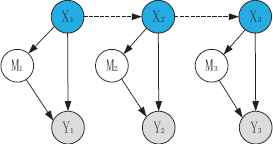
Structure of the GM-HMM.
In this study, the behavior estimation results are obtained according to the historic observation information, which can be expressed as follows:
2.2. Parameter learning of a specific network structure
Parameter learning means estimating the parameters of the conditional probability distributions of a specific network structure. Since there are hidden nodes in the network, this problem is considered partially observable. In this study, we define hidden parameters H = [Mt] and observable parameters O = [Yt, Xt]. Therefore, in the partially observable case, the log-likelihood is
The EM algorithm uses Jensens inequality26 to iteratively maximize.
According to Jensens inequality, for any concave function f,
Therefore, to maximize the low bound in the above equation with respect to q, it can be obtained that
The above step represents the E step. Maximizing the lower bound with respect to the free parameter θ′ is achieved by maximizing the following log-likelihood function:
This step is known as the M step. Dempster et al. proved that if θ′ is represented through Q(θ′|θ) > Q(θ|θ), one can guarantee that P(D|θ′) > P(D|θ), which improves the data log-likelihood25.
3. Distributed Genetic Algorithm Used to Optimize Structures
Because optimizing the structure of the network is a time consuming process, in this study, a distributed GA that can improve the network optimization speed is proposed. This section includes subsections namely analyzing the influence of structure on the models performance, GA and distributed GA used to optimize the models.
3.1. Influence of structure on the models performance
The structure of the network includes the intra-slice and inter-slice connectivities, which are represented by B1 and B→, respectively. Different structures of the network perform differently in order to understand the driving behavior.
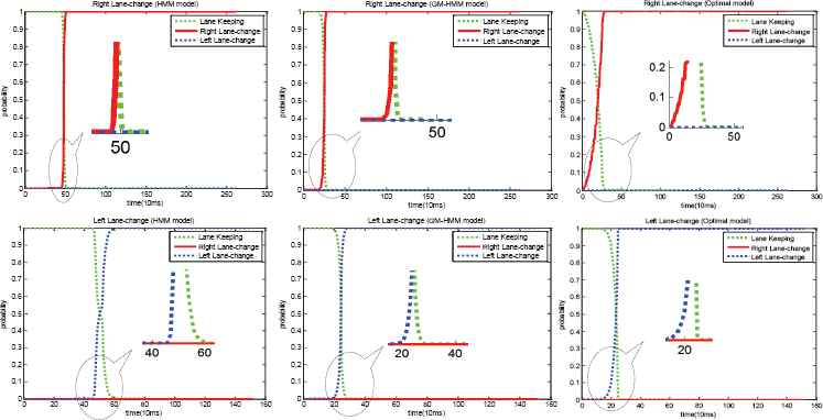
In this study, different intra, and inter-slice connectivities, and the parameters of hidden nodes together can lead to different networks with different performance. For example, in Fig. 3, if the parameter M is 1, then it equals the HMM. The inference results of GM-HMM, whose parameter M is defined as 3 for comparison, and HMM are shown in Fig. 4. In both models, there is a right and left lane change case. It is obvious that GM-HMM is much better than HMM with the same input data sequences because the GM-HMM model can estimate the behaviors earlier than the HMM model (The performance evaluation will be introduced in Section 4). Therefore, optimization of the network structure is significant in the DBA model.
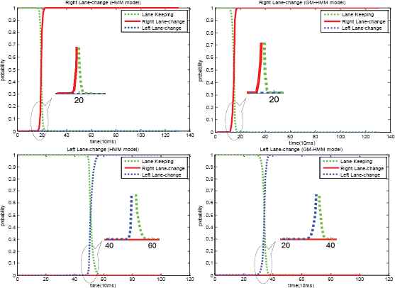
The estimation result comparison for two different models (HMM and GM-HMM) in two cases (right and left lane change case).
Since the optimization of the network structure is a non-linear problem, the GA is employed in this study. In addition, this algorithm is time consuming because of the EM algorithm; therefore, a distributed GA is employed. These algorithms will be introduced in the next two parts in this section.
3.2. Genetic algorithm to optimize the models
The term GA was first employed by Holland27. Now research into GAs is flourishing and goes much further than the original GA of Holland. A GA is a global search approach that mimics biological evolution28. GAs have several significant differences from other traditional optimization methods29. For example, it searches a population of points in parallel and not from a single point. Moreover, GAs do not require detailed knowledge about the problem but only the level of corresponding fitness according to the objective functions.
GAs are iterative toward to better solutions by applying the principle of fittest survival. Just as in natural selection, a new set of individuals will be created by a sequence of natural gene generations such as mating, mutation, selection according to their fitness level on the basis of problem domain, and recombination30–31.
3.2.1. The problem description
In this study, a GA is used to optimize the network structure. We assume that the structure of the network is a discrete search space χ, and the optimal function can be shown as follows:
3.2.2. The search space representation of networks
A network structure can be represented as an individual x, which conveys the DAG structure as well as the parameter in the hidden layer. The networks compose as two parts (B1, B→) as shown in Fig. 2; therefore, the individual x includes three parts as follows:
By considering the features of DAG24, g1 is defined as three binary strings:
g2, which represents the influential relationships for a two-slice temporal Bayes net B→, can be defined by nine binary strings:
g3, the gene of the hidden layer parameter, is defined as four binary strings in this study:
For example, the individual of HMM defined by a dynamic Bayesian network24 can be represented by the following equation:
As a result, there is a mapping from the individual x to the structure of the network s. Therefore, x could be given by the search space:
A population is formed by individuals of the networks that evolve by a set of actions such as selection, gene mating, recombination and gene muting. According to GA theory, the population can evolve into an optimal result, which means an optimized network structure. The evolution actions can be defined by the following equation:
However, this is a time consuming process because of EM algorithm at each alteration. In the following section, a distributed GA will be introduced, which could enhance the optimization speed based on the distributed algorithm.
3.3. Distributed genetic algorithm for optimization
In this section, a distributed GA for optimizing the network is proposed. A distributed system is defined as one in which the components from networked computers communicate and coordinate their actions by passing messages32. Distributed systems are widely used in web searches, online games, power system networks, etc. Furthermore, distributed systems have several advantages including being more reliable, more responsible, and less time consuming. These advantages were observed even when some distributed GAs were executed on a single processor33.
Several items influence the performance of the distributed GA, such as the number of demes, deme size, distributed topology of migration connection, migration intervals, migration rate, and other general genetic parameters. Several distributed topologies are widely used, as shown in Fig. 5. Master-slave is a simple model, which can evolve in a global way. In other distributed genetic topologies such as (b) and (c) in Fig. 5, good results will quickly migrate to all the demes with a dense connectivity. If the distributed genetic topologies are connected sparsely, the nodes will be more isolated and variable solutions will appear. In this study, a coarse grain and master-slave model is employed as the genetic topology which is a hybrid topology33. Here the individuals can migrate between directly adjacent demes as in Fig. 5 (c). Better individuals will be chosen as the better migrants replace the worse ones. More information about the influential items of GAs can be found in Cant-Paz35.
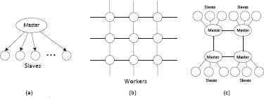
The connection topologies of some distributed genetic algorithm ((a) is a master-slave model, (b) is a fine grain model and (c) is a hybrid named coarse grain and master-slave model).
As a result, in the distributed GA for optimizing the networks, EM is used to learn the parameters in a specific network and the distributed GA is also employed to optimize the structure of the network. The algorithm can be briefly observed in Fig. 6.
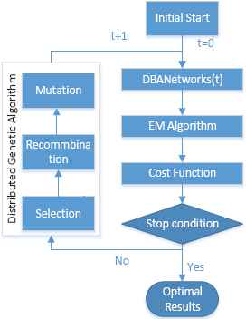
The DBA model based on the dynamic Bayesian network and distributed genetic algorithm.
4. Application in Lane-change Scenarios
In this study, the DBA model based on the dynamic Bayesian network and the distributed GA is applied to estimate the behaviors in vehicle lane-change scenarios. In addition, with V2V and V2I communication technologies, the traffic information can be shared. Then, the driving behavior of the around vehicles can be estimated using this modeling framework. This section first introduces the data collection. Then, the model based on the dynamic Bayesian network and distributed GA is used to learn the optimized solution to infer vehicle behaviors. Finally, the results are compared and analyzed.
4.1. Data collection
In this study, the estimating knowledge of the DBA model was learned from the naturalistic driving data. The database used in this research is for driving behaviors namely left and right lane-change and lane keeping. This scenario is shown in Fig. 7.
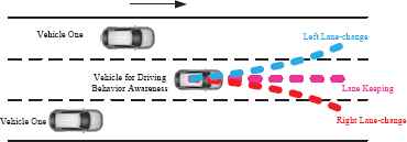
The vehicle lane-change scenario (including three lanes, and driving behavior in the middle lane was estimated).
The data collection experiment was conducted in Beijing, which included highways, ring road, airport express and normal city roads, shown in Fig. 8. The data collection includes approximately 18 km of road. Running information could be obtained by Controller Area Network (CAN), cameras and the LIDAR equipped on the data collecting vehicle. Running information, including the vehicles steering angle over time was stored. The data collection frequency was 100Hz. Fifty drivers that were asked to drive naturally and maintain their own driving styles.
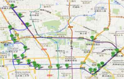
The data collection route. The data collection road is approximately 18 km, including highways, ring road, airport express and normal city roads.
From the collected data, the three behaviors mentioned above were labeled manually using the labeling graphical user interface (GUI) shown in Fig. 9. The information from LIDAR and cameras is displayed and the time serial information including the steering angle, lateral velocity and so on is represented by different color curves. These help determine the start and the end point of the lane-change case during the manual labeling process. The labeling procedures are as follows. Firstly, use the LIDAR map and images to mark the rough position of the lane-change case. Then, check and make sure that the velocity at the starting point should be greater than 30 km/h and the duration for lane-change should be lower than 8 s. Finally, the steering angle as well as lateral velocity are applied to label an accurate lane-change start and end time. Generally, the initial time of a cosine or sine curve is set to be the start time, and the first peak is set to be the end time36.
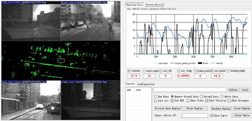
The labeling GUI. The left area displays the real time LIDAR map and images of the surrounding traffic environment. The top-right area shows the CAN data curves.
In this experiment, the detailed information about the database is introduced in Table 1. In this study, six hundred and thirty episodes were collected for the lane-change scenario, and four hundred and twenty-seven episodes chosen randomly from the database are applied as training cases and one hundred and eighty three as testing cases37.
| Labeled Behavior | Number | Gender | |
|---|---|---|---|
| Right Lane-change | 180 | Male | 61% |
| Female | 39% | ||
| Lane Keeping | 210 | Male | 71% |
| Female | 29% | ||
| Left Lane-change | 240 | Male | 55% |
| Female | 45% |
Detailed information about the database.
4.2. Evaluation index and cost function
In this subsection, evaluation indexes are proposed and defined, which can be used to evaluate the estimating performance and build the cost function for the distributed GA.
Definition 1.
Correct recognition is defined when the correct estimation is made with 90% or higher probability and incorrect recognition is defined when a wrong estimation is made with 90% or higher probability. From Fig. 10, the result for the right lane-change behavior is a correct recognition.
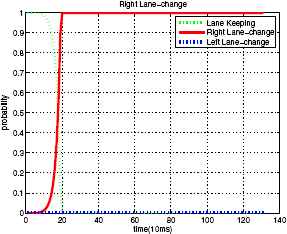
A case of the right lane-change estimation result. Time = 0 is the vehicle’s right lane-change starting point which is labeled manually, so tlabel = 0.
Definition 2.
Recognition succeed delay time, tsucceed, is defined as the time delay in the recognition succeed point, whereby, the recognition succeed point is defined to be the first point that the probability of the expected behavior estimation is equal or above 90% (t0.9). Recognition succeed delay time can be expressed as follows:
Definition 3.
Recognition start delay time, tstart, is defined as the time delay of the recognition start point, whereby, the recognition start point is defined to be the first point that the probability of the expected behavior estimation is equal or above 20% (t0.2). Recognition start delay time can be expressed as follows:
The purpose of defining this evaluation index, recognition start delay time, is to solve the condition in Fig. 11 and Fig. 12. In the two figures, the two models estimate the case of right lane-change behavior correctly (Definition 1) and almost at the same time (Definition 2). However, the time at which these two models start the estimation is different. Obviously, the second model starts to recognize earlier. In other words, the recognition start delay time of the second model is smaller.
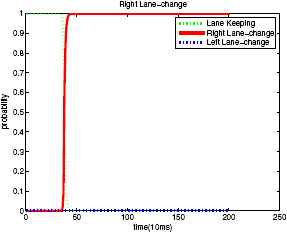
Estimating result of the first model.
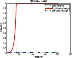
Estimating result of the second model.
The evaluation indexes defined above are used to evaluate a specific case of estimation. The indexes of recognition start delay time as well as recognition succeed delay time could reflect the sensibility or response of the models to the related behavior. Moreover, the evaluation indexes are crucial for AVs to make decisions based on the estimating models. The recognition start and succeed delay time for estimating driving behavior could influence the time to make decisions. In addition, the overall performance of the models can be verified and comprised using the average recognition start delay time, average recognition succeed delay time, correct recognition rate and incorrect recognition rate.
In this study, the cost function for the distributed GA is defined on the basis of evaluation indexes represented in the following equations:
4.3. Learning results
In this study, the configuration of the distributed GA is determined empirically38. Generally, the more individuals the population involves, the more chances to get the more superior results. However, more individuals lead to heavier computation cost and longer time of evolutions. The maximum generation represents the total iterations, which could be determined when the fitness remains constant or decrease a little as iteration generation increases39. According to the common settings of the GA or distributed GA, the parameters of the GA could be determined33–34,38. The maximum generation is 500, crossover probability is 0.8, mutation rate is 0.01, number of master demographics is 10, and size of each master demographics includes 30 individuals. The migration rate is 0.3 and the migration interval is 5 generations. All the demographics run on 10 desktop computers, each of which has 3 GHz CPU and has 4 processor cores with 8 GB RAM.
The optimized structure of the network is represented in Fig. 13. The parameter of the hidden node is 7. The given network structure means that the node in the behavior layer influences the hidden and observation nodes, and the hidden node has an impact on the observation node in the intra-slice Bayesian net. Furthermore, in the inter-slice Bayesian net, the behavior node at time t − 1 influences the behavior node at time t, and the hidden node at time t − 1 impacts the behavior and the observation nodes at time t.
The optimized structure of the network.
The average cost value with respect to the generation is shown in Fig. 14.
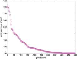
The cost value evaluation with generations.
4.4. Result comparison and analysis
In order to evaluate the estimation performance of the optimized network, this section compares the estimating results between the optimized networks with HMM and GM-HMM models, which were introduced in the previous sections. This comparison includes the analysis of specific cases and an average performance comparison.
First, two cases for right lane-change and left lane-change behaviors chosen randomly in the database for testing are evaluated using different models. With the same input information, the estimating results are shown in Fig. 15 and Table 2. In this figure, it can be concluded that the three models infer correctly in these two cases but their recognition succeed delay time and recognition start delay time are different. In both cases, the optimized model has the least recognition succeed delay time and recognition start delay time, which means that the optimized model has the best performance among the three models.
Estimating results of two cases in the database. One is left lane-change case and the other one is right lane-change. And they are estimated by three different models, namely, HMM, GM-HMM, and the optimized model.
| Recognition Result | Recognition Succeed Delay Time(s) | Recognition Start Delay Time(s) | |||||||
|---|---|---|---|---|---|---|---|---|---|
| HMM | GM-HMM | Optimal Model | HMM | GM-HMM | Optimal Model | HMM | GM-HMM | Optimal Model | |
| Right Lane-change case | Right | Right | Right | 0.50 | 0.27 | 0.26 | 0.48 | 0.25 | 0.13 |
| Left Lane-change case | Right | Right | Right | 0.55 | 0.26 | 0.25 | 0.48 | 0.24 | 0.22 |
Detailed information about the estimating results of two lane-change cases.
The estimating results of the testing database compared with HMM and GM-HMM are shown in Table 4. In the vehicle lane-change scenario, the optimal models average recognition rate is 93%. The average recognition succeed delay time is 0.19s and the average recognition start delay time is 0.17s.
| Recognition Result (%) | Average Recognition Succeed Delay Time(s) | Average Recognition Start Delay Time(s) | |||||
|---|---|---|---|---|---|---|---|
| RLC | LLC | LK | RLC | LLC | RLC | LLC | |
| HMM | 69 | 70 | 87 | 0.13 | 0.35 | 0.12 | 0.32 |
| GM-HMM | 94 | 87 | 88 | 0.10 | 0.29 | 0.09 | 0.27 |
| Optimized Model | 96 | 94 | 90 | 0.10 | 0.28 | 0.07 | 0.26 |
The average estimating performance analysis of the three models (RLC represents right lane-change, LLC represents left lane-change, and LK represents lane keeping).
5. Conclusions and Contributions
In this study, the DBA model based on a dynamic Bayesian network and distributed GA was built to estimate the behavior of vehicles in different traffic scenarios. There are three layers in the network, namely the observation, hidden, and behavior layer. The EM algorithm was employed to learn the parameters of a specific structure of the network. In order to optimize the structure efficiently, a distributed GA was designed using the hybrid coarse grain and master-slave topology. Then the proposed DBA model was applied in the vehicle lane-change scenario to estimate driving behaviors namely right lane-change, left lane-change and lane keeping. The performance evaluation index and cost function for a specific structure of the network were designed. In the vehicle lane-change scenario using the optimized model, the average recognition rate was 93%, the average recognition succeed delay time is 0.19 s and the average recognition start delay time is 0.17 s. Moreover, the estimating result of the optimized model was compared with other common models namely the HMM and GM-HMM. The comparison proved that the inference performance of the optimized model was much better than the two models.
An optimized structure for the DBA network was found to estimate the driving behavior, which is crucial for AVs to make decisions, particularly in complex traffic scenarios. In the future work, more information and the relationships between multiple vehicles will be included to improve the performance of DBA network proposed in this study.
Acknowledgments
This work was supported by the National Natural Science Foundation of China (Nos. 51475254 and 51625503), Junior Fellowships for Advanced Innovation Think-tank Program of China Association for Science and Technology (No.DXB-ZKQN-2017-035), Project funded by China Postdoctoral Science Foundation (No.2017M620765), the joint research project of Tsinghua University and Daimler, and the joint research project of Ministry of Education, China Mobile and Tsinghua University (No. MCM20150302).
References
Cite this article
TY  - JOUR
AU  - Guotao Xie
AU  - Hongbo Gao
AU  - Bin Huang
AU  - Lijun Qian
AU  - Jianqiang Wang
PY  - 2018
DA  - 2018/01/01
TI  - A Driving Behavior Awareness Model based on a Dynamic Bayesian Network and Distributed Genetic Algorithm
JO  - International Journal of Computational Intelligence Systems
SP  - 469
EP  - 482
VL  - 11
IS  - 1
SN  - 1875-6883
UR  - https://doi.org/10.2991/ijcis.11.1.35
DO  - 10.2991/ijcis.11.1.35
ID  - Xie2018
ER  -