
A locally weighted learning method based on a data gravitation model for multi-target regression
- DOI
- 10.2991/ijcis.11.1.22How to use a DOI?
- Keywords
- Multi-Target Regression; Locally Weighted Regression; Data Gravitation Approach
- Abstract
Locally weighted regression allows to adjust the regression models to nearby data of a query example. In this paper, a locally weighted regression method for the multi-target regression problem is proposed. A novel way of weighting data based on a data gravitation-based approach is presented. The process of weighting data does not need to decompose the multi-target data into several single-target problems. This weighted regression method can be used with any multi-target regressor as a local method to provide the target vector of a query example. The proposed method was assessed on the largest collection of multi-target regression datasets publicly available. The experimental stage showed that the performance of multi-target regressors can be significantly improved by means of fitting the models to local training data.
- Copyright
- © 2018, the Authors. Published by Atlantis Press.
- Open Access
- This is an open access article under the CC BY-NC license (http://creativecommons.org/licences/by-nc/4.0/).
1. Introduction
In the last decade, multi-target regression has gained the attention of the machine learning community, due to the numerous real-world problems that contain multi-target data. Particular applications involving multi-target regression include ecological modeling 25, chemometrics 16, automatic control 17, demography studies 38, energy efficiency 40, signal processing 42 and more.
Multi-target regression concerns the task of predicting multiple continuous variables using a common set of input variables 4,38. Multi-target regressors are commonly characterized by learning a global model to fit all of the training data. However, it is well known that the performance of a predictive model is quite related to the number and quality of training examples from which the model was constructed 43.
The overall performance of learning systems can be significantly improved by a proper local adjustment of their capacity (parameters of the learning algorithms) 43,5. Vapnik & Bottou 44 proposed the theoretical framework on which locally weighted learning is based; instead of fitting a model with all training examples, locally weighted learning methods fit a model to nearby data. Locally weighted learning is a form of lazy learning that aims to learn local models to fit the training data only in a region around the location of a query point 2. Examples of locally weighted learning methods include k-Nearest Neighbours (kNN) and Locally Weighted Regression methods.
Locally weighted regression allows to improve the overall performance of regression methods by adjusting the capacity of the models to the properties of the training data in each area of the input space 29. Locally weighted regression has been applied to numerous areas among which figure numerical analysis 26, sociology 49, economics 24, chemometrics 45, computer graphics 30, robot learning and control 36.
Locally weighted regression has been widely studied in single-target problems 29. However, to the best of our knowledge, locally weighted regression methods for multi-target regression problems have not been studied yet. In this paper, an effective local algorithm for multi-target regression, named as Locally Weighted Regression based on Data Gravitation (LWRDG), is presented. We propose a novel way of weighting data based on a data gravitation approach. Data gravitation approach comprises the application of physic gravitation principles to resolve machine learning problems 32. LWRDG directly weights the multi-target data, i.e. it does not decompose the multi-target problem into several single-target ones. It can be used with any multi-target regressor as a local method to provide the target vector of a query example.
To the best of our knowledge, this is the first attempt to study the benefit of the locally weighted regression to resolve multi-target regression problems in the machine learning area. Furthermore, for the first time, a data gravitation-based approach is applied to the locally weighted regression and multi-target regression problems. The results confirmed that the overall performance of multi-target regressors can be significantly improved by fitting the models to local training data in a region around the location of a query example.
An extensive experimental study was carried out on a collection of 18 datasets. It is the largest collection of benchmark multi-target regression datasets publicly available*. The proposed locally weighted learning method was assessed with the two most relevant multi-target regressors presented in the recent work Ref. 38. The experimental results were validated using non-parametric tests, as proposed in Ref. 9.
This paper is arranged as follows: Section 2 describes the multi-target regression problem, the most relevant multi-target regressors that have appeared in the literature, the basis of the locally weighted regression and data gravitation approaches. Section 3 presents LWRDG algorithm. Section 4 describes the experimental set-up and analyses the results. Finally, Section 5 provides some concluding remarks.
2. Preliminaries
In this section, the general definition of the multi-target regression problem is presented. The most relevant multi-target regression methods that have appeared in the literature are briefly discussed. The basis of the locally weighted regression and data gravitation approaches are also portrayed.
2.1. Multi-target regression problem
Let us say S is a dataset containing couples (x,y) where x ∈ 𝒳 is an input vector and y ∈ 𝒴 is a target vector. 𝒳 is the input space† containing d input variables (𝒳1, 𝒳2,…, 𝒳d), and 𝒴 is the output space‡ consisting of q target variables (𝒴1, 𝒴2,…, 𝒴q). Let us say xi is the input vector of the example i, and
Up to date, a large number of methods have been proposed to resolve multi-target regression problems. The taxonomy of multi-target regression algorithms can be organised into two groups: problem transformation methods and algorithm adaptation methods 4. Problem transformation methods transform a multi-target regression problem into several single-target regression problems. Then, for each resulting single-target problem, a classical regression method is executed, and finally, an aggregation strategy is performed. On the other side, the algorithm adaptation category comprises algorithms that are designed to directly handle multi-target data, i.e. they do not decompose a multi-target regression problem into several single-target regression problems.
Hoerl & Kennard 20 proposed the first work, as far as we know, regarding solve multi-target regression problem by means of a problem transformation method. The authors used the well-known one-versus-all baseline approach to perform a separate ridge regression for each individual target. Motivated by the tight connection between multi-target regression and multi-label classification problems, recent researches have been focused on applying some well-known problem transformations methods, that have been widely used in multi-label learning 14, to resolve multi-target regression problem. Spyromitros-Xioufis et al. 38 analysed how several multi-label approaches, such as the binary relevance, stacked generalization and classifier chains, are straightforward of applying in multi-target regression contexts. As for algorithm adaptation category, a large number of methods have been proposed, such as statistical methods 37, support vector machines 42,17, kernel approaches 3, multi-target regression trees 25, and rule-based methods 1.
Recently, Spyromitros-Xioufis et al. 38 conducted an extensive comparison between several state-of-the-art multi-target regressors. The authors showed that Stacked Single-Target (SST) and Ensembles of Regressor Chains (ERC) methods significantly outperform the baseline approach, which individually performs a single-target regressor for each target variable. The authors concluded that a superior performance can be attained by means of modelling potential statistical relationships between target variables. The results also showed that SST and ERC methods attain a better performance than several state-of-the-art multi-target regressors.
2.2. Locally weigthed regression
Locally weighted regression (LWR) attempts to fit the training data only in a region around the location of a query example. LWR is a type of lazy learning, therefore the processing of training data is often postponed until the target value of a query example needs to be predicted. LWR and kernel regression 31 are equivalent for data distributed on a regular grid away from any boundary. However, LWR outperforms kernel regression in irregular data distributions 2. LWR has an optimal rate of convergence in a minimax sense 39, and it has a high minimax efficiency among all possible estimators 12. Hastie & Loader 18 also demonstrated that LWR methods may handle a wide range of data distributions, and it can avoid boundary and cluster effects.
LWR depends on the distance function used to recover the nearest neighbours of a given query example. However, the distance function does not need to satisfy the formal mathematical requirements for a distance metric 2. LWR enables several ways to use a distance function 2, for instance: (I) one distance function is used in all parts of the input space (global distance function), (II) the parameters of a distance function are set for each query example by an optimization process (query-based local distance function), or (III) each training example has a distance function and its corresponding parameter values (point-based local distance function).
In LWR, weighting functions and smoothing parameters are also important issues. A weighting function (a.k.a. kernel function) computes the weight§ that has a neighbour of a query example. The maximum value of a weighting function should be at zero distance, and the function should decay smoothly as the distance increases. Examples of well-known weighting functions are Linear, Epanechnikov, Tricube, Inverse and Gaussian. Regarding smoothing parameters, a bandwidth parameter (h) defines the scale or range over which generalisation is performed. There are several ways to set the parameter h2, for instance by a fixed bandwidth selection, nearest neighbour bandwidth selection, global bandwidth selection, query-based local bandwidth selection or point-based local bandwidth selection. Cleveland & Loader 8 argued in favour of nearest neighbour bandwidth selection approach to fix the value of h; in this case, the parameter h is equal to the distance to the k-th nearest example.
2.3. Data gravitation approach
Data gravitation approach comprises the application of physic gravitation principles to resolve machine learning problems. To the best of our knowledge, Wright 48 was the first person in analysing clustering problems by mean of a gravitational approach. Later, Endo & Iwata 11 proposed a dynamic clustering algorithm which takes into account the global and local information of data, and Gómez et al. 15 presented a clustering algorithm which considers every example as an object in the input space.
As for classification tasks, several data gravitation-based algorithms have been proposed 32,7,46,33. Peng et al. 32 presented one of the most complete work concerning data gravitation-based classification. A set of data particles¶ are constructed from the original dataset. Given a query example, the gravitational force of each data particle to the example is computed. The gravitational field for each class is calculated according to the superposition principle, and the query example is classified according to the class with the highest gravitational field. Later, the method presented in Ref. 32 has been extended and improved by several methods proposed in Refs. 7, 33, 46.
Regarding regression tasks, to the best of our knowledge, the data gravitation approach has not been applied yet. We consider that the application of data gravitation could be effective to tackle the locally weighted regression in multi-target problem. Data gravitation-based models have demonstrated to be less sensitive in those cases where kNN methods severely deteriorate their performance; kNN methods tend to deteriorate their predictive performance on data with high dimensionality, non-separable classes, or non-uniform distribution of examples per classes 27. In this sense, Cano et al. 7 proposed a data gravitation model that outperforms several state-of-the-art kNN methods, and they also demonstrated its efficacy in imbalanced data. On the other hand, Reyes et al. 34 presented an effective data gravitation-based algorithm to solve the multi-label learning problem, a paradigm very close to multi-target regression.
3. Locally weighted learning method based on a data gravitation approach
A local regression can be applied to multi-target regression problem by (I) performing a locally weighted regression method for each target variable, or (II) designing a weighting method that directly handles the multi-target data. The main drawback of the first approach lies in the high computational cost in multi-target problems with a large number of target variables. In this work, we focused on the second approach; we designed a method for weighting data that does not need to decompose a multi-target problem into several single-target problems.
In this section, the basis of our proposal is presented. First, data gravitation-based concepts are presented. Second, the steps followed by our locally weighted learning method are explained.
Data gravitation-based model
As was discussed in Section 2.3, previous data gravitation-based works intend to construct an artificial data unit (called data particle) from several training examples. However, constructing artificial data particles from several examples have shown several disadvantages, leading to a significant degradation in the effectiveness of data gravitation-based methods 7,34. In this work, we followed the idea proposed in Refs. 7, 34, where each training example is considered as an atomic data particle.
Definition 1.
Atomic data particle. An atomic data particle is a data particle with a data mass equal to 1, i.e. the particle is formed by only one example. The centroid and target vectors of an atomic data particle are constituted by the original input and target vectors, respectively, of the corresponding example. An atomic data particle i is represented as a 3-tuple (xi,yi,wi), where xi is its input vector (position of the particle in the input space 𝒳), yi is its target vector (position in the output space 𝒴), and wi represents the numeric value of its neighbourhood-weight.
To simplify, hereafter the term atomic data particle is simply referred as particle. The concept of neighborhood-weight was firstly presented in Ref. 34, where the estimation process of the particle weights was inspired in the well-known extension of the ReliefF algorithm for regression problems 35. In this work, we reformulated the concept of neighbourhood-weight as follows:
Definition 2.
Neighbourhood-weight of a particle. The neighbourhood-weight of a particle i represents the probability of encountering particles in its neighbourhood with target vectors near the target vector of i.
Before to explain how to compute the neighbourhood-weight of a particle, we need to define some functions and probabilities. Given two particles i and j, the distance between their centroids is calculated as
Let us say Ni represents the k-nearest particles of particle i in the input space 𝒳. The prior probability that the k-nearest neighbours are far from i in the input space 𝒳 is computed as
The prior probability that the k-nearest neighbours are far from i in the output space given that they are far in the input space is computed as
Next, our locally weighted learning method is explained.
Locally weighted learning method
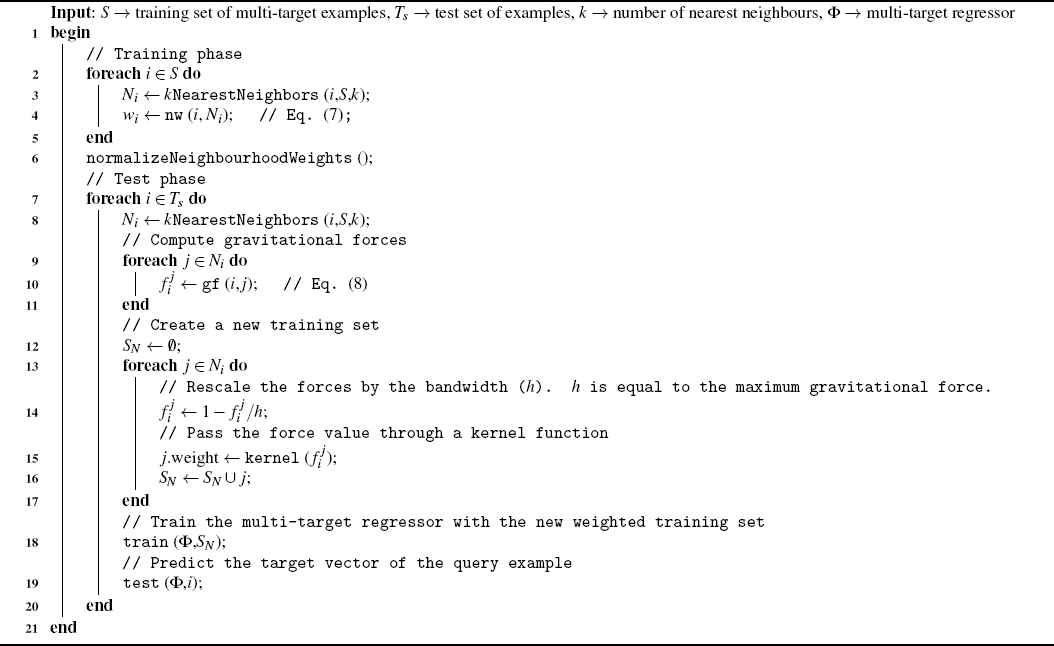
The steps followed by our locally weighted learning method are straightforward. The training phase is summarized in these three steps: (I) consider each training example i ∈ S as a particle, where S is a given training set, (II) compute the neighbourhood-weight of each particle i ∈ S, and (III) the neighbourhood-weight values of the particles are normalized to [0,1] range.
On the other hand, the test phase is summarized in these six steps: (I) given a query example i, the k-nearest particles of i are retrieved, (II) the gravitational forces between the query example i and each of the k-nearest particles are computed, (III) a weight for each nearest particle is computed by means of a kernel function using the gravitational forces, (IV) a weighted training set is composed by the k-nearest particles, (V) the weighted training set is used to train a multi-target regressor, and (VI) the induced model predicts the target vector of the query example i.
We named this approach as Locally Weighted Regression method based on a Data Gravitation model (LWRDG). Algorithm 1 shows the pseudo-code of the LWRDG method. LWRDG does not decompose the multi-target regression problem into several single-target problems, i.e. it directly handles the multi-target data. It can be used with any existing multi-target regression method as a local regressor to predict the target vector of query examples.
In the training phase, LWRDG needs to retrieve the k-nearest neighbours for each particle to compute neighbourhood-weight values. However, if the distance between each pair of training particles is pre-calculated and an adequate data structure for the searching process is employed, the computing of the k-nearest neighbours for each particle can be performed efficiently. Let us say fk is the cost function of searching the k-nearest neighbours of a particle. Therefore, in the training phase, LWRDG needs O(n · fk) steps, where n is the number of original training examples.
In the test phase, given a query example i, LWRDG retrieves the k-nearest particles to i, creates a weighted training set composed by the k-nearest particles, trains the multi-target regressor with the new weighted training set, and finally, predicts the target vector of the query example i. Let us say ftr(k,d,q) and fts(k,d,q) are the cost functions of training and testing, respectively, the multi-target regressor on a dataset with k examples, d input variables and q target variables. Therefore, the time complexity of LWRDG to predict the target vector of a query example is O(max(fk, ftr(k,d,q), fts(k,d,q))).
Note that, for multi-target regressors with slow training procedures, only k (k << n) examples are considered for training the regressor, leading to a notable improvement on the computational cost of these regressors. However, it is worthy to consider that this process is performed for each query example, since LWRDG algorithm is a lazy method.
LWRDG method.
4. Experimental study
This section presents a brief description of the multi-target regression datasets used in the experimental study, as well as describes how the effectiveness of our proposal was assessed.|| Finally, an analysis of the experimental results is depicted.
4.1. Multi-target regression datasets
In our experimental study, 18 multi-target regression datasets were used. To date, these 18 datasets constitute the largest collection of benchmark datasets for studying the multi-target regression problem38. Table 1 shows some statistics of the benchmark datasets. The datasets vary in size: from 49 up to 9803 examples, from 7 up to 576 input variables, and from 2 up to 16 target variables.
| Dataset | Source | n | d | q |
|---|---|---|---|---|
| andro | Ref. 19 | 49 | 30 | 6 |
| atp1d | Ref. 38 | 337 | 411 | 6 |
| atp7d | Ref. 38 | 296 | 411 | 6 |
| edm | Ref. 23 | 154 | 16 | 2 |
| enb | Ref. 40 | 768 | 8 | 2 |
| jura | Ref. 16 | 359 | 15 | 3 |
| oes10 | Ref. 38 | 403 | 298 | 16 |
| oes97 | Ref. 38 | 334 | 263 | 16 |
| osales | Ref. 21 | 639 | 413 | 12 |
| rf1 | Ref. 38 | 9125 | 64 | 8 |
| rf2 | Ref. 38 | 9125 | 576 | 8 |
| scm1d | Ref. 38 | 9803 | 280 | 16 |
| scm20d | Ref. 38 | 8966 | 61 | 16 |
| scpf | Ref. 22 | 1137 | 23 | 3 |
| sf1 | Ref. 28 | 323 | 10 | 3 |
| sf2 | Ref. 28 | 1066 | 10 | 3 |
| slump | Ref. 50 | 103 | 7 | 3 |
| wq | Ref. 10 | 1060 | 16 | 14 |
Statistics of the benchmark datasets (n: # of examples, # of input variables (d), # of target variables (q).
4.2. Experimental setting
In this work, the average Relative Root Mean Squared Error (aRRMSE) was employed to assess the effectiveness of our proposal. This evaluation measure has been commonly used to evaluate multi-target regression methods 1,38. In all experiments, to estimate the aRRMSE values a 10-fold cross validation was performed.
Let us say yi and ŷi are the vectors of the actual and predicted outputs for the example i, respectively. Let us say
As was previously described in Section 2.1, Spyromitros-Xioufis et al. 38 showed that SST and ERC regressors are significantly better than several state-of-the-art multi-target regressors. The authors conducted all experiments in the same 18 datasets used in this work, and they also demonstrated that these two multi-target regressors obtains the best results by using bagged 6 regression trees (BAG) as single-target base regressor (the predictions of 100 trees were combined). Consequently, in this work, our locally weighted learning algorithm was assessed with SST and ERC regressors. Hereafter, we dubbed the combination of SST and ERC methods with BAG as SST-BAG and ERC-BAG, respectively. Also, we refer to the combination of our proposal -LWRDG- with the SST-BAG and ERC-BAG local regressors as LWRDG-SST-BAG and LWRDG-ERC-BAG, respectively.
For the sake of fairness, for all lazy methods involved in the comparisons conducted, the best number of neighbours (k) was estimated via cross-validation. All computational methods were implemented in MULAN library 41. MULAN is a Java library which contains several algorithms, evaluation methods and measures for multi-label learning, and its functionality has been also expanded to support multi-target regression.
4.3. Results and discussion
Next, the results obtained in the different parts of the experimental study are presented and discussed.
4.3.1. Evaluating several kernel functions
The aim of this part of the experimental study was to evaluate the impact of several kernel functions on the overall performance of our proposal. LWRDG was analysed with the following five kernel functions:
- •
Linear: 1 − v
- •
Epanechnikov:
- •
Inverse: 1 / (1 + v)
- •
Tricube: (1 − v3)3
- •
Gaussian: e−v2
Table 2 shows the results of LWRDG-SST-BAG and LWRDG-ERC-BAG methods using the five kernel functions. The best error values are highlighted in bold typeface.
| Dataset | Linear | Epanechnikov | Tricube | Inverse | Gauss | Dataset | Linear | Epanechnikov | Tricube | Inverse | Gauss |
|---|---|---|---|---|---|---|---|---|---|---|---|
| andro | 0.470 | 0.475 | 0.472 | 0.475 | 0.478 | andro | 0.412 | 0.421 | 0.443 | 0.445 | 0.438 |
| atp1d | 0.383 | 0.383 | 0.375 | 0.384 | 0.382 | atp1d | 0.372 | 0.372 | 0.365 | 0.378 | 0.374 |
| atp7d | 0.526 | 0.532 | 0.523 | 0.540 | 0.537 | atp7d | 0.500 | 0.515 | 0.495 | 0.525 | 0.518 |
| edm | 0.728 | 0.727 | 0.728 | 0.728 | 0.727 | edm | 0.710 | 0.702 | 0.710 | 0.717 | 0.710 |
| enb | 0.133 | 0.132 | 0.132 | 0.138 | 0.137 | enb | 0.107 | 0.110 | 0.104 | 0.120 | 0.118 |
| jura | 0.599 | 0.600 | 0.599 | 0.600 | 0.599 | jura | 0.601 | 0.598 | 0.664 | 0.590 | 0.589 |
| oes10 | 0.422 | 0.422 | 0.422 | 0.422 | 0.422 | oes10 | 0.410 | 0.414 | 0.410 | 0.415 | 0.415 |
| oes97 | 0.523 | 0.524 | 0.523 | 0.524 | 0.524 | oes97 | 0.502 | 0.508 | 0.498 | 0.513 | 0.515 |
| osales | 0.741 | 0.748 | 0.746 | 0.747 | 0.748 | osales | 0.713 | 0.733 | 0.728 | 0.731 | 0.743 |
| rf1 | 0.171 | 0.171 | 0.171 | 0.171 | 0.171 | rf1 | 0.155 | 0.155 | 0.163 | 0.172 | 0.170 |
| rf2 | 0.319 | 0.357 | 0.312 | 0.318 | 0.322 | rf2 | 0.454 | 0.492 | 0.461 | 0.476 | 0.469 |
| scm1d | 0.322 | 0.322 | 0.322 | 0.322 | 0.322 | scm1d | 0.320 | 0.309 | 0.301 | 0.315 | 0.309 |
| scm20d | 0.348 | 0.349 | 0.348 | 0.349 | 0.349 | scm20d | 0.329 | 0.336 | 0.329 | 0.339 | 0.340 |
| scpf | 0.795 | 0.788 | 0.793 | 0.785 | 0.787 | scpf | 0.822 | 0.810 | 0.881 | 0.789 | 0.788 |
| sf1 | 1.069 | 1.061 | 1.073 | 0.972 | 0.983 | sf1 | 1.731 | 1.754 | 1.784 | 1.067 | 1.127 |
| sf2 | 0.985 | 0.978 | 0.989 | 0.981 | 0.984 | sf2 | 1.298 | 1.286 | 1.287 | 1.062 | 1.082 |
| slump | 0.705 | 0.700 | 0.711 | 0.702 | 0.703 | slump | 0.682 | 0.675 | 0.696 | 0.685 | 0.679 |
| wq | 0.913 | 0.913 | 0.912 | 0.914 | 0.914 | wq | 0.913 | 0.910 | 0.923 | 0.910 | 0.910 |
| Ave. rank | 2.833 | 3.028 | 2.583 | 3.306 | 3.250 | Ave. rank | 2.611 | 2.750 | 2.833 | 3.639 | 3.167 |
(a) Results of LWRDG-SST-BAG. The Friedman statistic, distributed according to χ2 with four degrees of freedom, is equal to 2.578. The p-value computed by Friedman’s test is equal to 0.631. The Friedman’s test did not reject the null hypothesis at a significance level α = 0.05.
(b) Results of LWRDG-ERC-BAG. The Friedman statistic, distributed according to χ2 with four degrees of freedom, is equal to 4.878. The p-value computed by Friedman’s test is equal to 0.300. The Friedman’s test did not reject the null hypothesis at a significance level α = 0.05.
Results of LWRDG using different kernel functions.
As a multiple comparison was conducted (every combination of LWRDG with a kernel function is considered as a different and independent method), the Friedman’s test 13 was performed to evaluate whether exist significant differences in the results. The last row in Table 2 shows the average ranks computed by Friedman’s test.
In both cases, i.e. studies with regards to LWRDG-SST-BAG and LWRDG-ERC-BAG, Friedman’s test did not detect significant differences in the results at the significance level α = 0.05. This means that, in average, our proposal had similar performances independently of the kernel function used. However, according to the average rankings computed by Friedman’s test, the LWRDG method obtained the lowest average ranks when using the Linear, Tricube and Epanechnikov kernel functions. These results are considered as good results, since they shows the stability of our data gravitation-based model, independently of the type of kernel function used to compute the weights.
4.3.2. Comparing with a well-known approach for weighting data
The aim of this part of the empirical study was to analyse whether our data gravitation-based model obtains superior performance than the basic approach for weighting data. The basic approach for weighting data (dubbed as BWR) is directly based on the distance values between a query example and its k-nearest neighbours; these distance values are used by the kernel functions to compute the respective weights. Consequently, two training examples at the same distance of a query example will have equal weights.
LWRDG and BWR methods were executed with the five kernel functions used in the previous Section 4.3.1. Tables 3 and 4 show the results using SST-BAG and ERC-BAG as local regressors, respectively. The best error values are highlighted in bold typeface.
| Dataset | Linear | Epanechnikov | Tricube | Inverse | Gauss | |||||
|---|---|---|---|---|---|---|---|---|---|---|
| LWRDG | BWR | LWRDG | BWR | LWRDG | BWR | LWRDG | BWR | LWRDG | BWR | |
| andro | 0.470 | 0.483 | 0.475 | 0.487 | 0.472 | 0.499 | 0.475 | 0.512 | 0.478 | 0.509 |
| atp1d | 0.383 | 0.391 | 0.383 | 0.390 | 0.375 | 0.392 | 0.384 | 0.392 | 0.382 | 0.410 |
| atp7d | 0.526 | 0.534 | 0.532 | 0.539 | 0.523 | 0.533 | 0.540 | 0.541 | 0.537 | 0.552 |
| edm | 0.728 | 0.751 | 0.727 | 0.751 | 0.728 | 0.750 | 0.728 | 0.751 | 0.727 | 0.751 |
| enb | 0.133 | 0.139 | 0.132 | 0.134 | 0.132 | 0.133 | 0.138 | 0.138 | 0.137 | 0.135 |
| jura | 0.599 | 0.603 | 0.600 | 0.603 | 0.599 | 0.603 | 0.600 | 0.603 | 0.599 | 0.621 |
| oes10 | 0.422 | 0.426 | 0.422 | 0.426 | 0.422 | 0.436 | 0.422 | 0.426 | 0.422 | 0.426 |
| oes97 | 0.523 | 0.530 | 0.524 | 0.530 | 0.523 | 0.530 | 0.524 | 0.531 | 0.524 | 0.531 |
| osales | 0.741 | 0.748 | 0.748 | 0.753 | 0.746 | 0.767 | 0.747 | 0.750 | 0.748 | 0.770 |
| rf1 | 0.171 | 0.183 | 0.171 | 0.176 | 0.171 | 0.184 | 0.171 | 0.176 | 0.171 | 0.176 |
| rf2 | 0.319 | 0.328 | 0.357 | 0.372 | 0.312 | 0.328 | 0.318 | 0.320 | 0.322 | 0.328 |
| scm1d | 0.322 | 0.325 | 0.322 | 0.325 | 0.322 | 0.325 | 0.322 | 0.325 | 0.322 | 0.325 |
| scm20d | 0.348 | 0.357 | 0.349 | 0.358 | 0.348 | 0.357 | 0.349 | 0.359 | 0.349 | 0.359 |
| scpf | 0.795 | 0.810 | 0.788 | 0.795 | 0.793 | 0.800 | 0.785 | 0.789 | 0.787 | 0.792 |
| sf1 | 1.069 | 1.134 | 1.061 | 1.033 | 1.073 | 1.092 | 0.972 | 0.973 | 0.983 | 0.992 |
| sf2 | 0.985 | 0.976 | 0.978 | 0.978 | 0.989 | 0.970 | 0.979 | 0.984 | 0.984 | 0.984 |
| slump | 0.705 | 0.713 | 0.700 | 0.715 | 0.711 | 0.726 | 0.702 | 0.709 | 0.703 | 0.711 |
| wq | 0.913 | 0.935 | 0.913 | 0.913 | 0.912 | 0.939 | 0.914 | 0.924 | 0.914 | 0.920 |
| p-value | 0.001 | 0.002 | 0.001 | 0.000 | 0.000 | |||||
Results of LWRDG-SST-BAG and BWR-SST-BAG methods using different kernel functions.
| Dataset | Linear | Epanechnikov | Tricube | Inverse | Gauss | |||||
|---|---|---|---|---|---|---|---|---|---|---|
| LWRDG | BWR | LWRDG | BWR | LWRDG | BWR | LWRDG | BWR | LWRDG | BWR | |
| andro | 0.412 | 0.425 | 0.421 | 0.455 | 0.443 | 0.462 | 0.445 | 0.499 | 0.438 | 0.456 |
| atp1d | 0.372 | 0.374 | 0.372 | 0.380 | 0.365 | 0.374 | 0.378 | 0.385 | 0.374 | 0.391 |
| atp7d | 0.500 | 0.504 | 0.515 | 0.523 | 0.495 | 0.498 | 0.525 | 0.549 | 0.518 | 0.530 |
| edm | 0.710 | 0.733 | 0.702 | 0.729 | 0.710 | 0.746 | 0.717 | 0.734 | 0.710 | 0.728 |
| enb | 0.107 | 0.109 | 0.110 | 0.111 | 0.104 | 0.105 | 0.120 | 0.122 | 0.118 | 0.159 |
| jura | 0.601 | 0.633 | 0.598 | 0.621 | 0.664 | 0.670 | 0.590 | 0.592 | 0.589 | 0.598 |
| oes10 | 0.410 | 0.423 | 0.414 | 0.417 | 0.410 | 0.412 | 0.415 | 0.434 | 0.415 | 0.418 |
| oes97 | 0.502 | 0.514 | 0.508 | 0.532 | 0.498 | 0.503 | 0.513 | 0.519 | 0.515 | 0.527 |
| osales | 0.713 | 0.729 | 0.733 | 0.742 | 0.728 | 0.733 | 0.731 | 0.754 | 0.743 | 0.773 |
| rf1 | 0.155 | 0.172 | 0.155 | 0.169 | 0.163 | 0.182 | 0.172 | 0.183 | 0.170 | 0.185 |
| rf2 | 0.454 | 0.467 | 0.492 | 0.545 | 0.461 | 0.536 | 0.476 | 0.483 | 0.469 | 0.451 |
| scm1d | 0.320 | 0.332 | 0.309 | 0.311 | 0.301 | 0.304 | 0.315 | 0.315 | 0.309 | 0.315 |
| scm20d | 0.329 | 0.341 | 0.336 | 0.344 | 0.329 | 0.338 | 0.339 | 0.347 | 0.340 | 0.352 |
| scpf | 0.822 | 0.844 | 0.810 | 0.825 | 0.881 | 0.892 | 0.789 | 0.794 | 0.788 | 0.794 |
| sf1 | 1.731 | 1.754 | 1.754 | 1.811 | 1.784 | 1.742 | 1.067 | 1.055 | 1.127 | 1.092 |
| sf2 | 1.298 | 1.189 | 1.286 | 1.180 | 1.287 | 1.189 | 1.062 | 1.070 | 1.082 | 1.154 |
| slump | 0.682 | 0.699 | 0.675 | 0.683 | 0.696 | 0.716 | 0.685 | 0.687 | 0.679 | 0.683 |
| wq | 0.913 | 0.915 | 0.910 | 0.918 | 0.923 | 0.987 | 0.910 | 0.925 | 0.910 | 0.934 |
| p-value | 0.002 | 0.002 | 0.011 | 0.001 | 0.005 | |||||
Results of LWRDG-ERC-BAG and BWR-ERC-BAG methods using different kernel functions.
We conducted a Wilcoxon signed-ranks test to determine whether LWRDG and BWR are statistically different using the same kernel function, as proposed by Demsar 9 for the statistical comparison between two independent algorithms. The p-values computed by Wilcoxon’s test are showed in the last row of Tables 3 and 4.
The results showed that LWRDG significantly outperformed to BWR method, independently of the kernel function used in the weighting process. In all cases, the Wilcoxon’s test rejected the null hypothesis at a significance level α = 0.05. The results confirmed that our data gravitation-based model can attain a superior performance in comparison with the weighting process that only considers the distance between examples.
4.3.3. Comparing local multi-target regression with global multi-target regression
The aim of this part of the experimental study was to analyse if our locally weighted regression method is able to outperform global multi-target regression methods, such as the SST-BAG and ERC-BAG regressors constructed with all training data. First, we compared a LWRDG-SST-BAG method with a SST-BAG regressor which was trained with all training data (dubbed as SST-BAG-Global). Second, we followed the same procedure, but a ERC-BAG regressor was used as a local regressor (LWRDG-ERC-BAG) and global regressor (dubbed as ERC-BAG-Global). To conduct the experiment, the Linear function was employed as kernel function.**
Table 5 shows the results of the experiment. The best error values are highlighted in bold type-face. We conducted a Wilcoxon’s test to compare the results obtained by SST-BAG, respectively ERC-BAG, as local and global regressor. The p-values computed by Wilcoxon’s test are showed in the last row of Table 5.
| Dataset | LWRDG-SST-BAG | SST-BAG-Global | Dataset | LWRDG-ERC-BAG | ERC-BAG-Global |
|---|---|---|---|---|---|
| andro | 0.470 | 0.603 | andro | 0.412 | 0.596 |
| atp1d | 0.383 | 0.398 | atp1d | 0.372 | 0.379 |
| atp7d | 0.526 | 0.561 | atp7d | 0.500 | 0.534 |
| edm | 0.728 | 0.747 | edm | 0.710 | 0.753 |
| enb | 0.133 | 0.145 | enb | 0.107 | 0.128 |
| jura | 0.599 | 0.612 | jura | 0.601 | 0.617 |
| oes10 | 0.422 | 0.428 | oes10 | 0.410 | 0.429 |
| oes97 | 0.523 | 0.526 | oes97 | 0.502 | 0.535 |
| osales | 0.741 | 0.751 | osales | 0.713 | 0.735 |
| rf1 | 0.171 | 0.197 | rf1 | 0.155 | 0.131 |
| rf2 | 0.319 | 0.123 | rf2 | 0.454 | 0.159 |
| scm1d | 0.322 | 0.360 | scm1d | 0.320 | 0.364 |
| scm20d | 0.348 | 0.493 | scm20d | 0.329 | 0.498 |
| scpf | 0.795 | 0.830 | scpf | 0.822 | 0.834 |
| sf1 | 1.069 | 1.141 | sf1 | 1.731 | 1.520 |
| sf2 | 0.985 | 1.112 | sf2 | 1.298 | 1.354 |
| slump | 0.705 | 0.732 | slump | 0.682 | 0.712 |
| wq | 0.913 | 0.917 | wq | 0.913 | 0.924 |
| p-value | 0.002 | p-value | 0.032 | ||
(a) LWRDG-SST-BAG vs. SST-BAG-Global.
(b) LWRDG-ERC-BAG vs. ERC-BAG-Global.
Comparing local multi-target regression with global multi-target regression.
Wilcoxon’s test rejected the null hypotheses at a significance level α = 0.05. It means that LWRDG was able to construct local models that significantly outperformed their global counterparts. The results suggested that a superior performance in the resolution of the multi-target regression problem can be attained by fitting the models to local training data in a region around the location of a query example.
4.3.4. Discussion
In this work, we used the HEOM distance function to search the k-nearest neighbours of a query example in the input space 𝒳. For future researches, it would be interesting to analyse the behaviour of our approach using other distance functions. In the study, five kernel functions were analysed, and we concluded that no exist clear evidence that the choice of the weighting function is critical for our approach. However, we observed that, in average, the best values were obtained when using the Linear, Tricube and Epanechnikov kernel functions (see Section 4.3.1).
The data gravitation-based model proposed was superior to the basic approach for weighting data that only considers the distance between a query point and its nearest neighbours (see Section 4.3.2).On the other hand, our model differs of traditional data gravitation-based methods in that it uses the concept of neighbourhood-weight to calculate gravitational forces. This coefficient increases or reduces the gravitational force of a particle over a query example. Two particles that are located in the input space at the same distance to a query point, but with different neighbourhood-weights, will have (I) different gravitational forces, (II) different weights computed by means of the kernel function, and therefore (III) different impacts in the final prediction of the target vector of the query point.
The results confirmed that multi-target regression methods can be significantly improved by only using local data around a query point (see Section 4.3.3). LWR methods do not have constraints regarding the regression method that can be used as a local regressor; it is worthy to note that the performance level of our proposal depends on the multi-target regression method used as a local regressor.
Based on the results and the statistical analysis conducted, we concluded that LWRDG method performed well in the resolution of the multi-target regression problem. The results also showed that our proposal can attain good performance levels on datasets with different properties.
5. Conclusions
In this work, a locally weighted learning algorithm for multi-target regression, named LWRDG, was proposed. LWRDG is based on the data gravitation approach, and it directly handles the multi-target data, i.e. it does not need to decompose a multi-target problem into several single-target problems. It considers each training example as an atomic data particle, avoiding the problems that may arise in the creation of artificial particles from various examples. It uses the neighborhood-weight concept that is employed in the gravitational force calculation instead of the particle’s mass. LWRDG can learn local models by using any multi-target regression method as a local regressor.
Our proposal was evaluated on 18 multi-target regression datasets. The experimental study confirmed the benefits of LWR methods to resolve the multi-target regression problem. The overall performance of multi-target regressors can be improved by fitting the models to training data only in a region around the location of a query point. On the other hand, the study showed the effectiveness of the data gravitation approach for the weighting process, as well as to conduct a LWR process on multi-target regression contexts.
Future research will study other approximations to adapt the data gravitation approach for resolving the multi-target regression problem. In this paper, we have focused on directly weighting the data. However, a promising research line is to study the effect of weighting the training criterion of the local model. Another interesting research line is to perform feature weighting and feature selection tasks into the local learning process. These tools would enable to tackle the curse of dimensionality in datasets with a large number of input variables.
Acknowledgements
This research was supported by the Spanish Ministry of Economy and Competitiveness and the European Regional Development Fund, project TIN-2014-55252-P.
Footnotes
The domain of input variables can be continuous, discrete or mixed type.
The domain of target variables is continuous.
The weight is considered the contribution of an individual point in a regression.
Data particle is a kind of data unit constructed from several training examples. A data particle has a data centroid and a data mass.
The algorithms and datasets are available to download at http://www.uco.es/grupos/kdis/kdiswiki/LWRDG.
According to the results presented in Section 4.3.1, not significant differences were encountered when using a different kernel function.
References
Cite this article
TY  - JOUR
AU  - Oscar Reyes
AU  - Alberto Cano
AU  - Habib M. Fardoun
AU  - Sebastián Ventura
PY  - 2018
DA  - 2018/01/01
TI  - A locally weighted learning method based on a data gravitation model for multi-target regression
JO  - International Journal of Computational Intelligence Systems
SP  - 282
EP  - 295
VL  - 11
IS  - 1
SN  - 1875-6883
UR  - https://doi.org/10.2991/ijcis.11.1.22
DO  - 10.2991/ijcis.11.1.22
ID  - Reyes2018
ER  -