
A Sparse Auto Encoder Deep Process Neural Network Model and its Application
- DOI
- 10.2991/ijcis.2017.10.1.74How to use a DOI?
- Keywords
- time-varying signal classification; process neural network; deep learning; SAE; training algorithm
- Abstract
Aiming at the problem of time-varying signal pattern classification, a sparse auto-encoder deep process neural network (SAE-DPNN) is proposed. The input of SAE-DPNN is time-varying process signal and the output is pattern category. It combines the time-varying signal classification method of process neural network (PNN) and the data feature extraction and hierarchical sparse representation mechanism of sparse automatic encoder (SAE). Based on the feedforward PNN model, SAE-DPNN is constructed by stacking the process neurons, SAE network and softmax classifier. It can maintain the time-sequence and structure of the input signal, express and synthesize the process distribution characteristics of multidimensional time-varying signals and their combinations. SAE-DPNN improves the identification of complex features and distinguishes between different types of signals, realizes the direct classification of time-varying signals. In this paper, the feature extraction and representation mechanism of time-varying signal in SAE-DPNN are analyzed, and a specific learning algorithm is given. The experimental results verify the effectiveness of the model and algorithm.
- Copyright
- © 2017, the Authors. Published by Atlantis Press.
- Open Access
- This is an open access article under the CC BY-NC license (http://creativecommons.org/licences/by-nc/4.0/).
1. Introduction
The classification of complex time-varying signals in nonlinear systems has always been an important issue in the field of signal processing and artificial intelligence. In practical engineering, due to the complexity of some nonlinear time-varying systems and the sampling signals are often affected by random factors, noise interference and some unknown factors, the sampled time-varying signals have a high degree of dependence on time changes, nonstationarity, high dimension, noise, modal features are variable and irregular and so on.1 In particular, the combination process features of multiple signals in multi-variable systems exhibit a high degree of complexity. To deal with this, signal processing techniques such as dimensionality reduction techniques, wavelet analysis or filtering can be applied.2 Expertise is also needed in selection of features and processing methods. The time-varying signal analysis model not only has to include more input nodes, but also has to memorize the past inputs. The length of the time-dependencies could be unknown, and the same input may be associated with different predictions.3 All of these problems present difficulties and challenges in the analysis and modeling of time-varying signal systems.
Some neural network models have been put forward to solve the signal processing in this kind of time-varying system, such as time delay neural network,4 recursive network,5 recurrent network,6 partial feedback network7 etc. In recent years, with the emergence of deep learning theory, some new network models have been proposed. Sepp Hochreiter and Jrgen Schmidhuber proposed a gradient-based long short-term memory (LSTM) in 1997. LSTM can achieve constant error flow through constant error carousels within special units. It is local in space and time.8 LSTM solves the complex tasks that the previous recurrent neural network (RNN) can not solve. In 2003, Michael and Peter use the dynamic behaviour of RNN to categorize input sequences into different specified classes. By adjusting the internal structure to represent the main features of the input sequence, so as to solve the classification problem. Its training speed and generalization ability significantly improved.9 In 2007, Sutskever and Hinton proposed a family of nonlinear sequence models. The idea is to use the undirected model for the interaction between hidden and visible variables. Multilevel representations of sequential data can be learned from the hidden layer, capture the effective modeling laws, improve the effect of the model by adding additional hidden layers. The model can be trained with high-dimensional, non-linear data.10 In 2008, Sutskever and Hinton et al. proposed a recurrent temporal restricted Boltzmann machine(RTRBM) for the modeling of natural data.11 TRBM is a probabilistic model for sequences that is able to accurately simulate complex probability distributions on high dimensional sequences. In 2010, Taylor and LeCun et al. proposed a model for studying the potential characteristics of image sequences from a pair of continuous images in order to learn better features to understand video data.12 The model can extract sensitive motion features from paired images, capture static and dynamic content, and the convolution architecture in the model can scale the model to the actual image size with compact parameterization. Deep convolution neural network (DCNN)13 has been widely used in image processing and speech recognition in recent years. DCNN uses image and timing data as input, through the multi-convolution, pooling, full connection operation, to achieve simplification, multilevel feature extraction and classification of complex sampling data.
Based on the above analysis, we can see that most of the neural network models used for analyzing the time-series signal are based on the existing static model. These models implement the input processing of the time-series signal by converting the time relationship into a spatial relation through extending the network input nodes (input dimension). By setting the memory storage unit in the network hidden layer, the recursive or cyclic information transmission and transformation strategy is used to realize the extraction and comprehensive analysis of the time characteristic. However, for complex multi-variable systems, intensive sampling data, or long time-series, this will make the network input layer and hidden layer presents a high dimension. At the same time, the information transfer process and the solving algorithm are also very complex. It is difficult to characterize and maintain the timing, relevance, and structural nature of the time-series sample data.
In 2000, in order to analyze the time-varying signal of nonlinear systems, He Xingui proposed14,15 a spatio-temporal information processing oriented process neural network (PNN). The process neuron structure differs from the traditional neuron in that its input and connection weights can all be time-varying functions, and an time-aggregation is added to the neurons. These can simultaneously express the interaction of multiple influencing factors and the accumulation of time effect. PNN is a feedforward network model composed of process neurons and the general non time-varying neurons according to certain topology and information transmission relationship. PNN represents and extracts the process characteristics of the time-varying signal by the connection weight function between the input layer and the hidden layer. It is an extension of the traditional artificial neural network in the time domain. Theoretical properties of PNN like the functional approximation ability of continuous time signal system, the continuity of the model and the existence of solution have been proved.4,16 PNN provides a new method for the analysis of time signals. It has been successfully applied in the field of time-varying signal classification,17,18 nonlinear time-varying system process simulation,19 and system state prediction and forecast20,21 etc. At present, some bottleneck problems still exist in the theoretical research and application of PNN, which mainly includes: (1) The existing PNN is a shallow structure model. Because of complexity of the process characteristics of nonlinear time-varying system signals, existing PNN models lack the ability of extraction, characterization and high-level synthesization for signal characteristics, which affects the accuracy of identification and discrimination of process characteristic details of complex signals; (2)The PNN model has many parameters. The selection of connection weights function and threshold has high degree of freedom. Under the condition that the training set is small and the expression of the system transforming characteristics is not complete, the generalization ability may be unstable; (3) There is no general method to design PNN algorithm, and the algorithm complexity is higher. It is difficult to realize the global optimization of many parameters based on the gradient algorithm. However, the deep learning theory provides an effective way to solve the above problems.
Deep Neural Network (DNN) is an artificial neural network model based on deep learning theory, put forward by G.Hinton, R.Salakhutdinov and other scholars in 2006.22,23 Due to its excellent ability of characteristic learning, training difficulty can be effectively overcome through layer-wise initialization algorithm based on unsupervised learning. The approximation of complex functions can be achieved by studying a deep nonlinear network structure. DNN has a strong ability of learning the essential features of the data set from a few samples, and has received widespread attention. It has been successfully applied in speech recognition24, machine translation,25 image processing,26 face recognition27 and many other fields. Deep Auto Encoder (DAE) is a typical model of deep learning structure, which is applicable for high dimensional complex data processing, and plays an important role in unsupervised learning and nonlinear characteristic extraction etc. In 1986, Rumelhart proposed the concept of Auto Encoder (AE)28 for processing of high dimensional complex data. In 2006, Hinton improved the prototype structure of auto encoder, and built a deep auto encoder model23, which firstly uses unsupervised layer-by-layer greedy algorithm to realize the pre-training of the hidden layer of DAE, and then uses BP algorithm to fine-tune the parameters of the whole neural network, which significantly improve the learning property and generalization ability of neural network. In 2007, Y.Benjio proposed Sparse Auto Encoder (SAE)29, which further deepens the research of deep auto encoder. It has a good property of signal dimension reduction. In 2012, Taylor deeply discussed the relationship between deep auto encoder and unsupervised characteristic learning, and established a general method for constructing different types of deep structure with auto encoder. In 2013, Telmo studied the performance of the deep auto encoder trained by different cost function, and pointed out the direction for the development of the optimization strategy of cost function.30 DAE can hierarchically present the learned features, it laid the foundation for construction deep structure. Therefore, a deep process neural network (DPNN) model and algorithm can be established by combining the dynamic information classification method of the process neuron network with the feature extraction and sparse representation mechanism of the deep automatic encoder. Problems in existing PNN research and application can be effectively overcome. At the same time, the information processing capability of the existing deep neural network can be extended to the time domain.
Aiming at the classification of nonlinear time-varying signal, this paper proposed a sparse auto encoder deep process neural network model (SAE-DPNN). It is constructed by stacking the process neuron hidden layer, McCulloch-Pitts neuron hidden layer, SAE network unit and softmax classifier. SAE-DPNN can not only express and synthesis the distribution features and combination process features of multi-variable nonlinear system in mechanism, but also can reflect the cumulative impact of process input. Under sparse constraint conditions, it can obtain relatively sparser and conciser feature matrix through deep learning, and increase the discrimination of different categories of time-varying signal samples, so as to realize direct classification of time-varying signal. In practice, due to the randomness of process distribution characteristics of the time-sampling signals, it is difficult to express it in an explicit form. In this paper, an implicit representation method based on orthogonal function base expansion is proposed. According to the statistical rules and distribution characteristics of the signal system, a set of appropriate standard orthogonal function basis is selected. The time-varying signal is expressed as a finite expansion of the function basis at a given fitting precision. Since each of the basis functions has definite morphological distribution characteristics, the process characteristics of the time signal function can be regarded as a linear combination of the basic characteristics of the group basis function, so as to realize the extraction and representation of the detail feature of the time-varying signals implicitly. Based on the existing SAE learning algorithm, a comprehensive training method based on orthogonal function basis expansion is established. Using the gradient-based algorithm with weight decay term to realize the initial training of parameter of PNN information unit in SAE-DPNN. Using unsupervised layer-by-layer initialization combining with teacher teaching to initialize the SAE parameters. And using the supervised BP algorithm to fine-tune the SAEDPNN parameters. Unlike existing deep network models, SAE-DPNN does not need to set the memory storage unit in the hidden layer. The input of the SAE-DPNN can be time-series signals or continuous time-varying functions. And the implicit expression of input time-varying signal is realized by using the algorithm strategy based on orthogonal function basis expansion. This method simplifies the network structure and information processing flow, and realizes the direct classification of the time-varying signals. Based on the time signal classification problem and the discrimination of reservoir water flooding condition based on well logging curve in petroleum geology research, simulation experiments were carried out. The results show that the model and algorithm are feasible and effective.
In this paper we review the challenges of time-varying signal classification, the status of artificial neural networks used for time-series signal processing, and point out the idea and algorithm of SAEDPNN. The SAE-DPNN model is established in Section 2, and its theoretical properties are analyzed. The learning algorithm of SAE-DPNN is given in Section 3. In Section 4, simulation experiments and result analysis are carried out to verify the feasibility and effectiveness of SAE-DPNN model and algorithm. Finally, conclusions are given in Section 5.
2. SAE-DPNN Model
In many time-varying signal processing problems, the multi-dimensional process signal distribution tends to be multi-modal, intersective, and complex due to the effects of various nonlinear disturbances, the coupling between signals, and the noise. Which shows a certain degree of multi-solution or ambiguity. It is difficult to identify the characteristics of the process signal. New models are expected to solve these problems. This new model should have a significant distinction between different types of signal synthesis characteristics. And can directly deal with a variety of time-varying process (function) signals. To solve these problems, this section establishes a sparse auto-encoder deep process neural network model.
2.1. Process neural networks
2.1.1. Process neurons
The process neuron, shown in Fig.1, consists of three parts, weighted sum of the input time-varying signals, aggregation of the spatio-temporal information, and the activation output. The inputs and connection weights can be time-related functions. Aggregation operation includes spatial aggregation and the accumulation of the time process effect of multiple input signals.
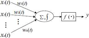
Model of process neuron.
In Fig.1, X(t) = (x1(t),x2(t), ⋯ ,xn(t))(t ∈ [0,T]) denotes the input vector of time-varying function. [0,T] denotes the interval of input signals. W(t) = (w1(t),w2(t), ⋯ ,wn(t)) denotes the corresponding connection weight functions. f denotes activation function of the process neuron. θ denotes the activation threshold. Σ denotes the spatial aggregation operator, taking weighted sum of multiple input signals. ∫ denotes the time aggregation operator for the process neurons, taking the integral operation of time. y denotes the output. The input/output relationship of the process neuron can be written as:
2.1.2. Process neural networks
The process neural networks is a feed-forward network model which is composed of a number of process neurons and McCulloch-Pitts(MP) neurons according to certain topological structure and the information transmission relationship. For conciseness, this paper only considers the multiinput/single-output system with one process neuron hidden layer. The networks topology is shown in Fig. 2.
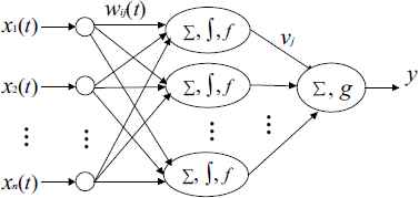
Model of process neuron networks.
By Fig.2, the input/output relationship of PNN can be written as:
In Eq.(2),
2.1.3. Double-hidden-layer process neural networks
Considering the information transmission relationship between PNN and SAE, a double-hidden-layer process neural network with single output is designed. The input layer and the first hidden layer are process neurons. The second hidden layer is MP neurons. The topology is as shown in Fig. 3. The process neuron hidden layer complete operations like extraction of the process features of time-varying input signals and spatio-temporal aggregation etc. The MP neuron hidden layer is mainly used to improve the networks mapping ability of the complex relationship between the input/output of the system, and to increase the knowledge storage capacity of the network.
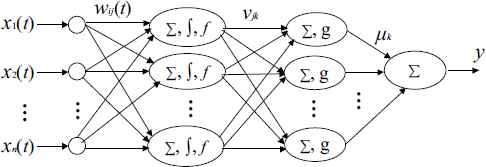
Double-hidden-layer process neural networks.
By Fig. 3, the input/output relationship of the double-hidden-layer process neural network can be written as:
In Eq. (3), vjk is the weight on the connection between the first hidden layer and the second hidden layer,
2.2. SAE-DPNN
The SAE-DPNN model is established by combining the PNN model with the properties of time-varying signal classification and the advantages of SAE network in data feature extraction and high-level sparse representation. Based on the double-hidden-layer process neural network model, a deep process neural network model with four layers of information units was constructed by stacking: time-varying process signal input layer, process neuron hidden layer, sparse deep auto encoder structure, and classifier as output unit.
2.2.1. Auto-Encoder
The auto encoder (AE) is a symmetrical three-layer neural network, which is composed of input layer, hidden layer and output layer, as shown in Fig. 4. First, the input data is encoded by the hidden layer, then the input data is reconstructed by the hidden layer, and the reconstruction error is minimized to obtain the best expression and feature extraction of data hidden layer.
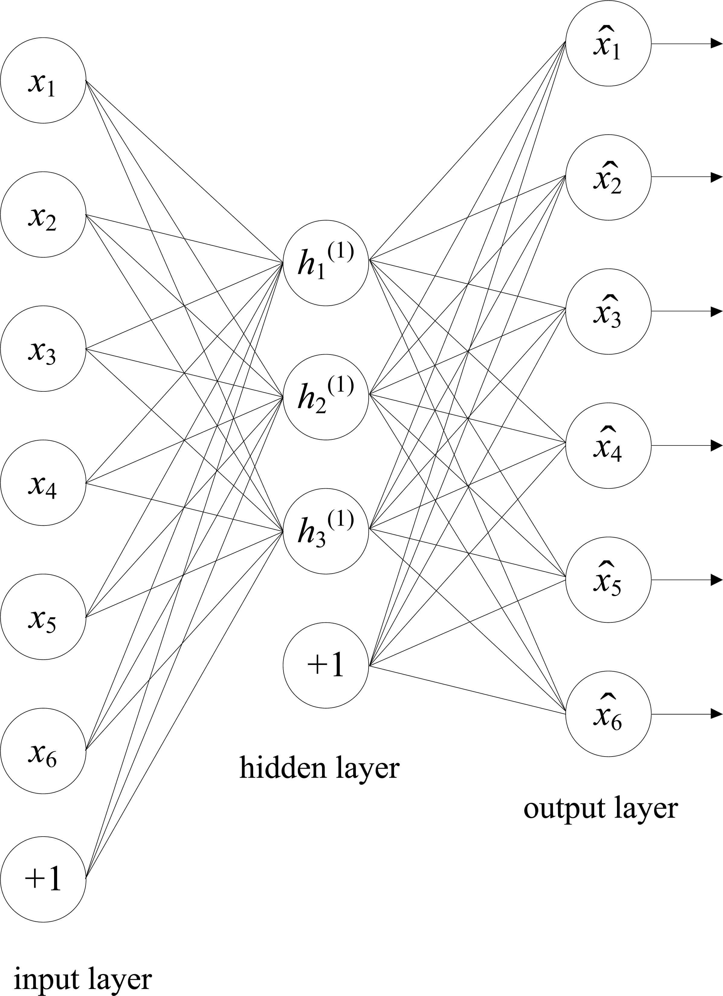
Structure of auto encoder.
The goal of auto encoder learning is to make the output of the network as approximate as possible to the input, and the training process consists of the encoding process and the decoding process. In the encoding process, the input samples are linearly mapped and nonlinearly transformed to be expressed by the hidden layer. Suppose
The decoding process is to re-project the encoded data to the original signal space, and obtain the decoded signal
The goal of auto encoder training is to make the decoding output as approximate as possible to the input before encoding. The network parameters are optimized by minimizing the reconstructing error, and the cost function is defined as follows:
After training of an auto encoder, the activation value of the hidden layer is used as the input of the next auto encoder. By this way, the multiple layers of auto encoder are stacked up to form an stacked auto-encoder.
2.2.2. Sparse Auto-Encoder
The Sparse Auto-Encoder uses the idea of sparse coding, introducing sparse penalty term on the basis of auto encoder. It can obtain relatively sparser and conciser data features through learning under sparsely constrained conditions.
Based on the stacked auto-encoder model, a sparse penalty term is added to the cost function to control the number of activated neurons in the hidden layer. If the neuron’s output is approximate to 1, it is considered that the neuron is “active”; on the contrary, it is considered as “inactive”. One of the goals of the sparse encoder is to make the hidden layer neurons to be “inactiv” in most of the time. Assuming that aj(x) represents the jth activated unit of the hidden layer. For the N training samples, in the forward propagation process, the average activation of the jth unit of the hidden layer is
Since it is desirable that most of the neurons are “inactive” the average activation quantity ρj should approximate to a constant ρ, which approximates to zero. ρ is a sparse parameter.
In order to achieve the sparse object, the penalty term is added to the cost function of the encoder to penalize ρj so that it can not deviate from ρ. The Kullback-Leibler (KL) divergence31 is used to define the penalty term PN, the expression is:
Penalty term is determined according to the nature of KL divergence: if ρj = ρ, KL(ρ∥ρj) = 0; else the KL divergence value will gradually increase with the deviation of ρj from ρ. Therefore, when the sparse penalty term is added, the network cost function of the sparse auto-encoder can be defined as:
2.2.3. SAE-DPNN model
Based on double-hidden-layer process neural network, a generalized 4-layer deep process neural network model composed of time-varying signal input layer, the hidden layer of process neurons, SAE deep structure unit, and softmax classifier was given, as shown in Fig. 5.
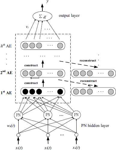
Model of SAE-DPNN
In Fig.5, there are n input nodes, m nodes in the process neuron hidden layer , and K nodes in the MP neuron hidden layer. The part from the input layer to the MP neurons hidden layer is the information processing unit of PNN. It is used to complete the input of n-dimensional time-varying signals x1(t),x2(t), ⋯ ,xn(t)(t ∈ [0,T]) to the network, and spatial and temporal weighted aggregation of the input signals, it’s outputs are
According to Fig.5, the input/output relationship of SAE-DPNN can be written as follows:
- (1)
The input/output relationship of the double-hidden-layer PNN
Input: x1(t),x2(t), ⋯ ,xn(t)t ∈ [0,T]
Output:
where, f1 and f2 are activation functions of process neurons and MP neurons, respectively.
- (2)
The input/output relationship of SAE
Input:
Output:
- (3)
The input/output relationship of the softmax classifier units
where, f3 is the activation function of the softmax classifier. θ is the threshold.
Comprehensive above all, the input/output relationship of SAE-DPNN can be written as:
In the application, the number of hidden layers of PNN and SAE structural units can be selected according to the dimension of time-varying input signal, the size of training sample set and the complexity of signal system.
3. Learning Algorithm of SAE-DPNN
Since the inputs of SAE-DPNN can be multidimensional process signals, the process neuron includes space-weighted aggregation and time effect cumulative two kinds of operators, the computation is of high complexity. In this paper, considering the signal transmission relationship between the information units of PNN and SAE network, the time-varying input signals and the connection weight functions are expressed by a set of orthogonal function bases. This method can reduce the complexity of process neuron space-time aggregation, and realize the implicit representation of time-varying signal process features based on function basis.
The learning process of SAE-DPNN is divided into 4 stages. The first stage is pre-processing. Select an appropriate set of standard orthogonal function basis and expansion method in time-varying function space. Finitely expand the sample functions in training set under the given fitting accuracy. At the same time, express the connection weight functions as a linear combinations of the same set of function basis. In stage 2, the initial values of connection weights between hidden layers of the double-hidden-layer PNN in Fig. 3 are trained. And use the results as the initial values of PNN information unit parameters in SAE-DPNN. In stage 3, use the output of the second hidden layer of double-hidden-layer PNN as the input of SAE. Based on unsupervised layer-by-layer initialization strategy and teacher teaching, initialize the parameters of SAE and softmax classifier. In stage 4, use BP algorithm to fine-tune the SAE-DPNN parameters.
3.1. Spatio-temporal aggregate operations of process neuron based on orthogonal function basis expansion
Suppose the input space of the process neural network is (C[0,T])n. b1(t),b2(t), ⋯ , bl(t) is a set of standard orthonormal function basis in C[0,T]. X(t) = (x1(t),x2(t), ⋯ , xn(t)) is the time-varying signal function in C[0,T]. Given the fitting accuracy, xi(t) can be expressed as the finite expansion of the function basis:
In Eq.(15),
That is,
As b1(t),b2(t), ⋯ ,bL(t) is a set of standard orthogonal basis functions in [0,T], Eq.(16) can be simplified as
3.2. Initialization training of PNN connection weight parameters
Substituting Eq.(17) into Eq.(3), the input/output relationship of the double-hidden-layer PNN can be expressed as:
Given P learning sample functions:(xp1(t),xp2(t), ⋯ , xpn(t),dp), p = 1,2, ⋯ , P. The first sub p of xp1(t) represents the sequence number of the learning sample, and the second sub i denotes the component number of the input function vector. dp is the expected output corresponding to the input xp1(t),xp2(t), ⋯ , xpn(t). Suppose yp is the actual output corresponding to the input xp1(t),xp2(t), ⋯ , xpn(t). Seen from Eq.(3), the learning error function can be defined as
In Eq.(19),
The gradient-based algorithm with weighted decay term is applied to the initialization training of the connection weights and threshold parameters of the double-hidden-layer PNN. The cost function is defined as:
The correction formulas of the connection weights and activation threshold of double-hidden-layer PNN are as follows:
3.3. Pre-training of SAE units
According to the cost function of SAE defined by Eq. (10), the pre-training of SAE units will eventually need to obtain optimized connection weights W and the bias b. And the sparse cost function Csparse is a function with W and b as parameters, the optimal W and b are obtained by minimizing the sparse cost function through back propagation algorithm.26 Using the batch training method, the gradient is used to update the weights once in each iteration. The update equations are as follows:
In this way, by calculating the average activation, the penalty term in the cost function is obtained. By optimizing the sparse cost function to get a better sparse representation of the hidden layer.
3.4. Training steps of SAE-DPNN
SAE-DPNN training includes four main steps: initialization training of double-hidden layer PNN based on gradient descent algorithm; layer-by-layer initialization training of SAE based on unsupervised greedy learning; initialization softmax classifier; according to the category labels in training set samples function, fine-tune the parameters in SAE-DPNN by using BP algorithm. The algorithm steps are as follows:
- step 1:
initialization training of PNN;
- step 1.1:
set the error accuracy ε1 > 0, the cumulative learning number s1, the maximum learning number M1, select the standard orthogonal basis function b1(t),b2(t), ⋯ ,bL(t), express the time-varying input function xi(t) and the connection weight function wi j(t) as the expansion of the function basis;
- step 1.2:
initialize weights and threshold parameters,
- step 1.3:
calculate error function E defined by Eq.(9), if E < ε1 or s1 > M1, then goto step1.5;
- step 1.4:
- step 1.5:
output learning result, end.
- step 1.1:
- step 2:
use error control or iterative number control strategy to initialize the SAE;
- step 2.1:
set K the hidden layer number of the SAE deep structure unit, m1 the number of input/output layer nodes for a single SAE unit, number of hidden nodes m2, the error accuracy ε2 > 0, and the maximum learning number M2;
- step 2.2:
take the output of the second hidden layer of the PNN that completes the initialization training as the input of the first SAE unit;
- step 2.3:
- step 2.4:
If the training stop condition is satisfied, then goto step 2.5; else goto step 2.3;
- step 2.5:
store the learning results, and proceed to the next SAE unit training until the deep SAE training is completed.
- step 2.1:
- step 3:
initialize softmax classifier parameter;
- step 4:
Given the training error ε3 or the maximum number of iterations M3, the BP algorithm is used to fine-tune the overall parameters of SAE-DPNN.
4. Simulation Experiments and Result Analysis
Example 1 Nonlinear time-varying function classification problem
Consider the pattern classification problems of the following 4 classes of time-varying functions. The sample functions are respectively defined as:
When λ = 0.85,the typical sample function curves and the characteristic distribution are shown in Fig. 6.
Curves of 4 classes sample functions.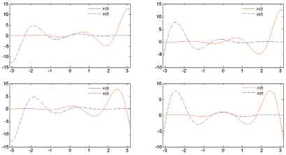
In each class, the value of λ is respectively 0.05,0.1,0.15,0.2, ⋯ ,1.0. Each class can get 20 function samples, forming a sample set containing 80 samples. The expected outputs of the 4 kinds of sample functions are respectively set as 0,1,2,3. Chose trigonometric function basis {1, cos t, sin t, cos 2 t, sin 3 t, ⋯ , cos nt, sin nt, ⋯} as the basis expansion function system. The orthogonal interval is [−π,π]. Expand the 80 sample functions under the fitting precision of 0.01. When the number of expansion terms is 33, it meets the fitting accuracy. Using a 4-fold cross-fold validation experiment, 80 sample functions were randomly divided into 4 groups, 3 groups as training set and 1 group as test set. Four sets of training and test samples were obtained. And take the average of 4 training and test results as the evaluation index. Structure and learning parameters of SAE-DPNN are selected as follows: Time-varying signal system has two variables, so SAE-DPNN take two input nodes. Other parameters were determined by experimental comparative analysis. Of which, 20 process neurons in the first hidden layer, 130 non-time-varying neurons in the second hidden layer; SAE information unit is constructed by stacking 4 SAE components, the number of units in input layer and output layer are both 130, and the number of hidden units are both 30; sparse penalty term weight β takes 0.035, SAE pre-training learning rate ε takes 0.55, other learning parameters take 0.5; 1 output node in softmax classifier. The structural parameters of SAE-DPNN are shown in Table 1. Use the algorithm constructed in section 3 to train SAE-DPNN. According to the algorithm given in section 3.2, the initialization training of the double-hidden-layer PNN unites are conducted under the accuracy of 0.05, and its convergent after 1022 times of iteration. Use the output of the second hidden layer units of the double-hidden-layer PNN as the inputs the information units of SAE; the number of SAE training times is 1000; the SAE-DPNN global tuning training iteration number is set to 1200 times; training error accuracy takes 0.05. The computer is configured to Intel Core i5-3470, CPU@3.2GHz, 4GB memory, WIN7 32 bit operating system in this experiment; simulation environment is Maltlab 2012. Through the learning of function samples in the training set, the classification model of SAE-DPNN is established, the error curve of training is shown in Fig. 7. The results are as follows: for 60 training samples, the training time was 37.623s, the average approximation error of the 60 samples in training set is 0.00972, discriminant accuracy rate is 100%; for 20 test samples, average approximation error is 0.01563, the correct recognition rate is100%.
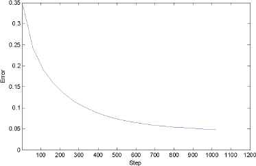
Error curve of SAE-DPNN fine-tune training.
| PN unit |
SAE unit |
Softmax classifier |
||||||
|---|---|---|---|---|---|---|---|---|
| input nodes | PN hidden nodes | MP hidden nodes | input nodes | hidden nodes | output nodes | hidden layers | input nodes | output nodes |
| 2 | 20 | 130 | 130 | 30 | 130 | 9 | 130 | 1 |
Structural parameters of SAE-DPNN.
As a comparison, process neural networks(PNN),32 double-hidden-layer PNN(DH-PNN),33 radial basis function process neural network RFBPNN34(the kernel function is Gauss function), the network structure parameter setting is shown in Table 2. And the SAE-DPNN model and algorithm established in this paper are used to conduct 10 times of initialization comparison experiments. The training error is set to 0.05. The results are shown in Table 3.
| PNN |
DH-PNN |
RBFPNN |
|||||||
|---|---|---|---|---|---|---|---|---|---|
| input nodes | hidden nodes | output nodes | input nodes | hidden layer nodes | second hidden layer nodes | output nodes | input nodes | hidden nodes | output nodes |
| 2 | 20 | 1 | 2 | 20 | 130 | 1 | 2 | 20 | 1 |
Structural parameters of the networks.
| serial number | algorithm | training set |
test set |
|||
|---|---|---|---|---|---|---|
| average time | approximation error | recognition rate | approximation error | recognition rate | ||
| 1 | PNN | 9.756s | 0.0477 | 100% | 0.0836 | 78.6% |
| 2 | DH-PNN | 12.720s | 0.0276 | 100% | 0.0492 | 82.7% |
| 3 | RBFPNN | 9.692s | 0.0374 | 100% | 0.0733 | 80.2% |
| 4 | SAE-DPNN | 34.223s | 0.0152 | 100% | 0.0262 | 100% |
Comparison of training indexes of different models.
In Table 3, the average approximation error is calculated by the following formula:
Known from Table 3, the average approximation error of test set and training set, the correct recognition of the training set of SAE-DPNN model and algorithm established in this paper is much better than the other three models and algorithms. This is because the combination of the two input functions of each sample in the training set is similar, and the sample set is small and incomplete. PNN, DH-PNN and RBFPNN are shallow models. Their small sample modeling capabilities, generalization capabilities, and distinguishing the characteristics of the sample category are not as good as SAE-DPNN. So, SAE-DPNN achieved better results. However, the SAE-DPNN algorithm is of high complexity and takes longer training time, but its time cost is worthy comparing with the obvious increasing of approximation error and correct recognition rate.
Example 2 Identification of logging flooded layer in petroleum development geology research.
Reservoir water flooding condition identification is a very important and complicated work in oilfield development. At present, the interpretation of water flooding layer is mostly based on the corresponding relationship between the electrochemical characteristics of the flooded reservoir, physical properties of rocks and logging response curve. When the reservoir is flooded, its physical properties, underground fluid properties and pore structure parameters will be complicatedly changed, its difficult to get the accurate value. In the existing automatic identification method, there are many problems such as the low coincidence rate of the discriminant model and the actual situation, and the difficulty of extracting the characteristics of the logging curve pattern.35 The author uses SEA-DPNN as the discriminator, automatically identify the reservoir flooded condition based on the characteristics of logging curve.
The identification of sublayer water flooding condition in well logging is based on the morphology and amplitude distribution of multiple logging curves which reflect the deep continuous sampling of drilling profile and reflecting the physical properties change of rock and fluid of drilling section, and the combinations among them. Different sedimentary units and fluid properties have different physical properties, which reflect different model characteristics of logging curves. This experiment studies oilfield geological block of fluvial delta deposit. Self potential SP, 2.5m resistivity R25, the microelectrode difference (Rmt-Rmd), natural gamma GR, acoustic AC, and the thickness of sand body h are selected as features to identify water flooding condition. Water flooding degree is divided into four levels, strong water flooding, medium water flooding, weak water flooding and non water flooding. According to the results of the analysis of the core wells and the results of expert interpretation, 4 kinds of 300 well logging flooding pattern samples were selected in proportion as the training set. Typical sample curves are shown in Fig. 8.
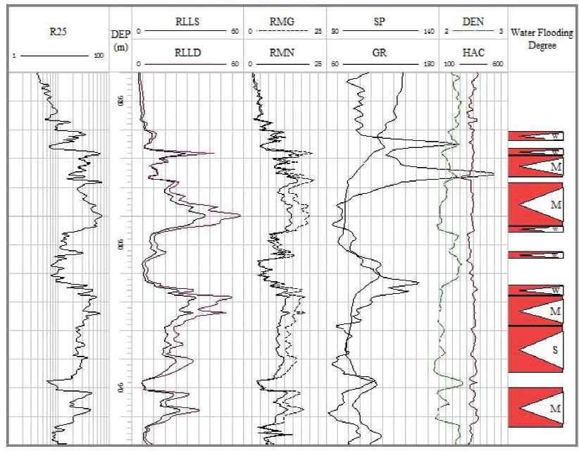
Typical log response characteristics of typical small water flooding pattern.
When SAE-DPNN is used to identify the reservoir flooding condition, the input process interval must be uniformed and the logging data must be standardized. In the actual data processing process, generally each sublayer’s thickness is different, so the input process interval is not consolidated. Rounded the maximum thickness of all the small layers of the well to be treated, and add 1 to constitute a consolidated process interval. In this way, the thickness variable of the sublayers has been implied in other input functions, so the thickness parameter can be removed. At the same time, the logging indexes are different in dimension, and the magnitude difference is large. The formula:
The training set is consists of 300 reservoir logging flooded samples selected from coring wells, SAE-DPNN as classifier, the normalized reservoir logging curves are used as network inputs, the output is the water flooding level. Leyrand function basis is used to fit the data of sublayer well logging, and the precision is set to 0.01. When the number of Legendre function basis terms is 7, the fitting accuracy is satisfied. The experimental results show that the SAE-DPNN architecture is chosen as follows: 5 time-varying input signals; in PNN information units, the first hidden layer with 20 units, the second hidden layer with 100 units; the number of input units in the SAE is 100, the number of hidden layer is 8, the number of hidden units is 20, and the output units number is 100; 1 softmax classifier output unit. SAE-DPNN is trained by the sample functions. The initialization training of double-hidden-layer PNN units is convergent after 1720 times of iteration under precision of 0.05; the output of the second hidden unit of PNN is used as the input of the SAE network, the number of training times is 800, and the global optimization training of SAE-DPNN is set to 1000. The trained SAE-DPNN was used as the reservoir water flooding level identification model. The accuracy rate is 100% for the training samples. For 227 samples(i.e. test set) of 15 uncored wells, comparing with the expert manual evaluation results, automatic recognition consistent rate reaches 92.7%. Under the same conditions, a 5-20-1 process neuron network, a 5-20-100-1 double hidden layer process neuron network, a 5-20-1 radial basis function process neural network (the kernel function is Gauss function) were adopted. The correct recognition rate of the test set was 79.3%, 86.3% and 83.7%, respectively. SAE-DPNN also achieved good results in the practical application. This is due to the number of factors in the development of oilfields is large, the characteristics of logging curves and the relationship between them are complex, and the training sample set is not complete. These affects the generalization ability of each model. Compared to other models, SAE-DPNN has the best properties.
5. Conclusion
Aiming at the problem of complex time-varying signals pattern classification in nonlinear system, this paper proposes and establishes a deep process neural network model based on the combination of sparse auto encoder and process neural network. The input of the SAE-DPNN can be time-series signals or continuous time-varying functions. The PNN unit can be used to initialize the extraction and representation of the signal process features. Unlike existing deep network models in dealing with time-series signals, SAE-DPNN does not need to set the memory storage unit in the hidden layer. So that the time-series signal can be maintained forward processing, simplifying the network information processing. At the same time, the algorithm based on orthogonal function base expansion is used to transform the process feature identification and analysis of the signal into the comparison between the expansion coefficients under the same set of orthogonal function basis, which simplifies the computational complexity of the model. SAE-DPNN has high level of synthesis and sparse representation of data process features, which improves the generalization ability and classification accuracy of the model. But SAE-DPNN training sample set needs to have better completeness and larger scale. The computational complexity is also high, and the choice of network parameters has a high degree of freedom. These are the issues that need further study. The experimental results show that the model and algorithm provide a feasible analysis model and algorithm for dynamic signal pattern classification.
References
Cite this article
TY  - JOUR
AU  - Xu Shaohua
AU  - Xue Jiwei
AU  - Li Xuegui
PY  - 2017
DA  - 2017/07/28
TI  - A Sparse Auto Encoder Deep Process Neural Network Model and its Application
JO  - International Journal of Computational Intelligence Systems
SP  - 1116
EP  - 1131
VL  - 10
IS  - 1
SN  - 1875-6883
UR  - https://doi.org/10.2991/ijcis.2017.10.1.74
DO  - 10.2991/ijcis.2017.10.1.74
ID  - Shaohua2017
ER  -