
Interval-valued Evidence Updating with Reliability and Sensitivity Analysis for Fault Diagnosis
- DOI
- 10.1080/18756891.2016.1175808How to use a DOI?
- Keywords
- Fault diagnosis; interval-valued belief structures; Dempster-Shafer evidence theory; evidence updating; alarm monitoring
- Abstract
Information fusion methods based on Dempster-Shafer evidence theory (DST) have been widely used in fault diagnosis. In DST-based methods, the monitoring information collected from sensors is modeled as multiple pieces of diagnosis evidence in the form of basic belief assignment (BBA), and Dempster’s rule is then used to combine these BBAs to obtain the fused BBA for diagnosis decision making. However, the belief structure with crisp single-valued belief degrees in BBA may be too coarse to truthfully represent detailed fault information. Moreover, Dempster’s rule only uses a static combination process, which is unsuitable for dynamically fusing information collected at different time steps. In order to address these issues, the paper proposes a dynamic diagnosis method based on interval-valued evidential updating. First of all, the diagnosis evidence is constructed as an interval-valued belief structure (IBS), which provides a more informative scheme than BBA to model fault information. Secondly, the proposed evidential updating strategy can generate updated IBS as global diagnosis evidence by updating the previous evidence with the new incoming evidence recursively. Thirdly, the reliability and sensitivity indices are designed to evaluate and compare the performance of the proposed updating strategy with other commonly used strategies. Finally, the effectiveness of the proposed evidential updating strategy is demonstrated through some typical fault experiments of a machine rotor.
- Copyright
- © 2016. the authors. Co-published by Atlantis Press and Taylor & Francis
- Open Access
- This is an open access article under the CC BY-NC license (http://creativecommons.org/licences/by-nc/4.0/).
1. Introduction
Fault diagnosis depends on multi sensors to monitor whether the behavior of an industrial system is correct, which is a main way of alarm monitoring in an industrial alarm system. Information collected from multi-sensors have to be fused together because normally a single sensor may not be able to get sufficient information for fault diagnosis. In practical situation, data collected by most sensors are inherently uncertain, imprecise or even incomplete due to various factors, such as random environmental disturbances, sensor instrument errors, etc1. Therefore, it is imperative to design a fusion mechanism for minimizing the effects of such imprecision and uncertainty on diagnosis decisions. Dempster-Shafer evidence theory (DST) is known to be capable of dealing with this kind of uncertain information fusion. DST can robustly deal with incomplete data and allows the representation of both imprecision and uncertainty2. It provides Dempster’s rule of combination to fuse multi-source information so as to reduce the effects of the uncertainty and yield more accurate diagnosis results. Therefore, DST has already been widely used in fault diagnosis of typical industrial systems under uncertain environment, such as rotating machinery3–4, power electronics5–6, control system7–8, sensor network 9 and so on.
Commonly, there are three interrelated steps for establishing a DST-based diagnosis system. The first step is to set up a frame of discernment (FoD) consisting of fault hypotheses. Different hypotheses in the FoD indicate different diagnosis goals. For instance, if we only want to detect whether a system is normal or abnormal, we may construct the FoD as Θ={F0, F} in which the system state is described to be either faulty F or normal F0. In order to differentiate a specific fault from the others, the FoD can be expanded to Θ={F0, F1,…, FN}, where Fi signifies the presence of the ith fault mode. If we further need to detailedly analyze the severity level of a specific fault, we may set Θ={SL(slight), MO (moderate), SE(severe)}. The second step is to obtain a basic belief assignment (BBA) function, in which the belief degrees, i.e., belief masses, are used to measure the extent to which that on-line monitoring information supports each diagnosis hypothesis and the subsets of the hypotheses. Such a BBA can also be also named as a piece of diagnosis evidence. There are different ways for generating BBAs from different types of information and data collected by sensors or even extracted from experts’ experiences. The typical ways include fuzzy matching10, neural network 5, decision tree 5, artificial immune algorithm 4, expert system 7 and so on. The final step is to choose appropriate combination rules to fuse these BBAs and make a diagnosis decision according to the fused results. Besides Dempster’s rule, some improved combination rules have also been given to handle conflicting diagnosis evidence 7,11.
Although these methodological contributions have stimulated the application of DST in the area of fault diagnosis, the current DST-based diagnosis mechanism has some inherent defects worthy of further analysis and discussion:
- •
The belief structure with crisp single-valued belief degrees in BBA may be too coarse to truthfully represent detailed fault information. Therefore, Simple crisp belief structure may miss or distort useful fault information which may lead to incorrect diagnosis decision 12.
- •
The fusion mechanism of Dempster’s and other improved rules are “symmetric” or “static” 13–14, and they are usually suitable for fusing multiple BBAs locally collected at the same time step. However, in order to support reliable decision-making, on-line diagnosis further requires aggregating the newly fused BBA at the current time step with the old results accumulated in the past dynamically. Obviously, the relationship between the new and old results is dissymmetric, so the previous rules may be no longer applicable.
- •
Correct detection rate and false alarms rate are commonly used indices for evaluating the performance of a diagnosis algorithm 5, but this kind of “hard” indices rarely reflects how “close” the fused BBA is to the true situation. Particularly, while taking both symmetric and dissymmetric fusing processes into consideration, we need to design other comprehensive performance indices satisfying soft and dynamic requirements.
The first point above is concerned with the representation of uncertainty. In recent years, interval-valued belief structures (IBSs) have attracted considerable attention for its effectiveness of modeling and combining uncertain information by using interval form of belief masses15–17. Compared with single-valued BBA, IBS can describe fault information in a more elaborate way and caters for human’s general understandings to uncertainty. Ref.12 presented a fuzzy feature extraction and matching method to generate the IBSs for fault diagnosis from multi-source data, and then fused them using the optimal combination rule for interval evidence proposed in Ref.15. Using the same set of data, Ref.12 also generated BBAs and fused them. A number of comparative studies on a machine rotor system proved that IBS captures more useful fault information from uncertain data than BBA and can enhance accuracy of DST-based diagnosis system.
The second point is concerned with the dynamic updating of diagnosis knowledge. The available diagnosis information can be classified into two parts. One is the previous knowledge base that has been constructed from a vast amount of evidence accumulated at the past steps, and the other is the diagnosis evidence gathered at the current time step. Generally speaking, the former may contain more comprehensive diagnosis information than the latter, but in a dynamically changing environment the new incoming evidence may reflect the current state of the system more accurately. Thus we should introduce an updating process to update the previous knowledge base with the new knowledge according to the human’s common-sense reasoning mechanism and utilize the knowledge from both parts for making a comprehensive diagnosis decision. The diagnosis decision according to the updated knowledge should be more credible than that derived from either of the two parts. As the contributions of two parts to the updated knowledge are different or dissymmetric, some updating strategies different from symmetric combination rules need to be introduced for combining the two parts effectively.
Some scholars have devoted their efforts to theoretical research of the updating strategies in different ways. Ref.18 and Ref.19 presented Jeffrey’s rule of conditioning and transferable belief model respectively. Ref.14 re-interpreted Jeffrey’s rule and gave a Jeffreylike rule for updating basic belief assignment function. Ref.20 gave the linear updating rule to combine the new BBA with the previous BBA. It was concluded in Ref.13 that “updating is a subtle operation and there is no single method, no single ‘good’ rule. The choice of the appropriate rule must always be given due consideration.” The same is true for dynamic diagnosis, and the above theoretical methods are rarely completely applicable. For example, the updated results gave by the Jeffrey-like rule are excessively determined by the current diagnosis evidence 1. The linear updating rule is effective, but how to set the linear combination weights of evidence is an open question 1.
The third point is about the performance evaluation of a diagnosis algorithm. The diagnosis decision making of a DST/IBSs-based diagnosis system is based on some principles of maximum belief degree, maximum plausibility, maximum of pignistic probability, etc21. For instance, suppose there are two fused BBA denoted as m⊕,I and m⊕,II coming from algorithm I and algorithm II respectively. If m⊕,I(F1)=0.6, m⊕,I(F2)=0.4, m⊕,II(F1)=0.9, m⊕,II(F2)=0.1, then, according to the principles of maximum belief degree, both of them can give the “hard” judgment that fault F1 happens. However, it is obvious that algorithm II is more credible because m⊕,II(F1) is closer to the definite solution “m(F1)=1” than m⊕,I(F1). Once this “distance” to the solution is quantified, the progress that an algorithm makes becomes observable as it converges on the solution22. In particular, when developing a dynamic updating process for diagnosis evidence, we have to synthetically consider the degree and speed of the convergence. While much research is being carried out to develop new fusion algorithms for fault diagnosis, limited research has been conducted to design indices for evaluating their static and dynamic performance.
In order to address the three concerns outlined above, this paper presents a new linear updating strategy of IBSs for on-line diagnosis, and also designs corresponding performance indices to assess and compare different updating methods on a commonly used diagnosis problem. Firstly, the Euclidean distance of evidence is extended to the framework of IBSs. Secondly, a new linear updating rule of IBSs is proposed to recursively generate the current updated IBS by updating the previous IBS with the new incoming IBS. In the updating process, similarity between the two IBSs is produced from the proposed distance and used to calculate the linear combination weights. A diagnosis decision is then made using the updated diagnosis evidence. Thirdly, based on the similarity, the static reliability index (SRI) and dynamic sensitivity index (DSI) are designed to measure the convergence degree and speed of the updating diagnosis algorithms respectively.
The rest of this paper is organized as follows. Section 2 reviews the relevant concepts of DST and IBSs. Section 3 introduces the extended Euclidean distance between two IBSs. Section 4 presents the new linear updating strategy of IBSs for on-line fault diagnosis. Section 5 designs the static reliability index (SRI) and dynamic sensitivity index (DSI). Section 6 reports that a few comparative experiments of dynamic fault diagnosis in a machine rotor system show the capacity of SRI and DSI and the applicability of the proposed linear updating strategy for diagnosing faulty states of the rotating machinery. The conclusions are presented in section 7.
2. Review of relevant concepts
2.1. Basic of DST
Let Θ be a finite set of elements. Each element in Θ can be a hypothesis, an object, or a fault in our case. We refer to Θ as the frame of discernment. Correspondingly the set consisting of all the subsets of Θ is called the power set of Θ, which can be denoted as 2Θ.
A function m: 2Θ → [0,1] is called a mass function if it satisfies the following two conditions: m(∅) = 0 and ∑A∈2Θ m(A)=1. This function is also named as basic belief assignment (BBA) or belief structure. A subset A with a non-null mass is viewed as a focal element. Commonly, if an information source can provide a mass function on Θ, this mass function is called a body of evidence, abbreviated to evidence.
The belief function (Bel) and Plausibility measure (Pl) can be defined as follows:
Bel measures the confidence granted to A and all subset of A, and Pl measures the confidence that A cannot be refused.
If m1, m2 are two BBAs induced from two independent information sources, a combined BBA can be obtained by using Dempster’s combination rule
Note that the Dempster’s combination rule is meaningful only when ∑B∩C=∅m1(B)m2(C) < 1, i.e., m1 and m2 are not completely conflicting. This rule can be used to aggregate uncertain, imprecise or incomplete information coming from different sources.
Let m be a BBA on Θ. Its Pignistic probability function BetPm: Θ→0,1] is defined as23
2.2. Basic of IBS
In an IBS, belief masses are no longer described by crisp numbers, but lie within certain intervals. It is constrained as follows.
Definition 115
Let A1,…,AN be N subsets of Θ and [ai-,ai+] be N intervals with 0≤ai-≤ai+≤1, i=1,2,…,N, an interval-valued belief structure (IBS) is defined as a set of BBAs such that the following conditions hold:
- (1)
- (2)
- (3)
m(H) = 0, ∀H ∉ {A1,…,AN}
According to the above definition, each subset Ai such that ai+>0 is called a focal element of an IBS. If
Definition 2 15,
If the ai- and ai+ of a valid IBS m satisfy respectively
An original IBS may be only valid, but not normalized, so Ref.24 gave a normalization formula as
A valid IBS can be normalized by using the above inequality. Table 1 gives an example to illustrate the normalization process. Here, m1 is a valid IBS because it satisfies the conditions in Definition 1, but it is not normalized according to Definition 2. Hence, Eq.(5) is used to normalize m1 so as to obtain the valid and normalized IBS m2 by cutting some infeasible subintervals of m1. In the following, we assume that an IBS is valid and normalized, unless it is stated explicitly.
| {θ1} | {θ2} | {θ3} | {Θ} | |
|---|---|---|---|---|
| m1 | [0.5,0.8] | [0.2,0.35] | [0.0,0.05] | [0.2,0.4] |
| m2 | [0.5,0.6] | [0.2,0.3] | [0.0,0.05] | [0.2,0.3] |
The normalization of valid IBS
After BBA is extended to IBS, the following important work is to combine two or multiple IBSs.
Definition 315
Let m1 and m2 be two IBSs with the intervals of belief masses [ai-,ai+] (ai-≤m1(Ai)≤ai+, i=1,2,…,N1) and [bj-,bj+] (bj-≤m2(Aj)≤bj+, j=1,2,…,N2) respectively. Their combination, denoted as m1⊕m2, is also an IBS defined by
For instance, Table 2 gives two IBSs m1, m2 and m1 ⊕ m2. Obviously, like Dempster combination rule, the combination rule of IBSs can also reduce uncertainty and converge belief mass to the focal element simultaneously supported by m1 and m2. Referring to Ref.15, the combination of two IBSs in Definition 3 can also be extended to the situation of multiple IBSs.
| {θ1} | {θ2} | {θ3} | Θ={θ1,θ2,θ3} | |
|---|---|---|---|---|
| m1 | [0.6,0.7] | [0.05,0.15] | [0.0,0.01] | [0.2,0.3] |
| m2 | [0.55,0.65] | [0.05,0.15] | [0.0,0.01] | [0.25,0.35] |
| m1 ⊕ m2 | [0.78,0.89] | [0.03,0.13] | [0.0,0.01] | [0.06,0.12] |
The fused IBS by combination rule
Actually, if any m(Ai) in an IBS m satisfies the constraint
3. The Euclidean distance between IBSs
Before presenting the Euclidean distance of two IBSs, we need to clarify the geometrical interpretation for IBSs.
Definition 427
An interval number X in ℜ is defined as the set of real numbers such that X=[x-,x+]={x’ ∈ ℜ : x-≤x≤x+}. X is degenerated iff x-=x+. Each degenerated interval number [x-=x, x+=x] can be treated as the real number x.
Definition 527
Denote the set of all close intervals X in ℜ as Int(ℜ) (the subset of 2ℜ). Vector V=(X1, X2,…, Xn)T (n∈N) is defined as an interval-valued vector in (Int(ℜ))n built of n elements Xi=[xi-,xi+]={ xi’ ∈ ℜ : xi- ≤ xi’ ≤ xi+}.
Vector V is an extension by replacing elements being crisp numbers with elements being intervals in a vector. Each classic vector is a special case of an interval-valued vector where its each element is a degenerated interval.
According to Definition 4 and Definition 5, we obtain:
Definition 6
Let m be an IBS with the intervals of belief masses [ai-,ai+] (ai-≤m(Ai)≤ai+, i=1,2,…,2|Θ|), thus, m is defined as an interval-valued vector in a multi-dimensional space Ω=Int1(ℜ) × Int2(ℜ) ×…× IntN(ℜ), N=2|Θ|, such that Inti(ℜ) is the space of intervals of belief masses of Ai ⊆ Θ and the element [ai-,ai+] in Inti(ℜ) satisfies the valid and normalized requirements in Definition 1 and Definition 2 respectively.
For example, Θ={θ1, θ2}, an IBS is given by m({θ1}) ∈ [0.2, 0.4], m({θ2}) ∈ [0.4, 0.7], m({θ1, θ2}) ∈ [0, 0.3]. The subsets of Θ are ordered as A1={∅}, A2={θ1}, A3={θ2}, A4={ θ1, θ2}, thus this IBS is an interval-valued vector m=([0,0], [0.2,0.4], [0.4,0.7], [0,0.3])T in space Ω=IntA1 (ℜ) × IntA2 (ℜ) ×IntA3 (ℜ) × IntA4 (ℜ).
We set Θ={θk| k=1,2,…,n}, where n=|Θ| denotes the cardinality of Θ, namely, the number of elements of Θ. Following the spirit of optimization in Definition 3, we can define the extended Pignistic probability function of m as
Actually, the extended Pignistic transformation projects the mass intervals of subsets of Θ into a new orthogonal space Ω′=Intθ1 (ℜ) × Intθ2 (ℜ) ×…× Intθn (ℜ).
In the orthogonal space Ω′, we use normalized Euclidean distance to measure the dissimilarity between the interval-valued vectors IBetPm1 and IBetPm2.
Definition 7
Suppose m1, m2 are two IBSs on Θ, and their corresponding Pignistic probability functions are IBetPm1 and IBetPm2 respectively. The extended Euclidean distance between IBetPs of two IBSs can be defined as
Obviously, the larger d(IBetPm1, IBetPm2) is, the more different m1 and m2 are, and vice versa, so d can be used to indirectly measure the dissimilarity between m1 and m2. We will rigorously check that d is indeed a metric distance in Lemma 1.
4. The linear updating of IBS for dynamic fault diagnosis
Essentially, Dempster’s rule and other symmetric combination rules can only provide static fused results, as they are just used to fuse several pieces of diagnosis evidence appearing at the same time step. As a result, the diagnosis decisions based on the fused results are also static. However, the running states of the equipment being monitored usually changes dynamically. Therefore, there are two main variations should be considered in diagnosis1 :1) Even if an equipment works in a normal state, intermittent or abrupt external disturbances are sometimes so strong that the static fusion methods may temporarily make false judgments. Actually, these disturbances never lead to the internal faults of the equipment; In this case, a perfect fusion method should always make the correct (i.e., no fault) judgments; 2) the equipment may undergo a gradual change from the normal status to a certain fault, or may abruptly jump from the normal status to a certain fault. In this case, a perfect fusion method should make prompt and stable responses to the changes.
In order to deal with dynamic diagnosis, next we introduce the linear updating rule of evidence presented in Ref.20 and further extend it to IBSs. The updated IBS recursively generated by the extended rule can integrate the current static fused IBSs with the previous updated IBSs so as to make a global and stable judgment.
4.1. The linear updating rule of interval-valued structures
In Ref.28, Fagin et al. defined the notions of conditional belief and plausibility functions. For any two focal elements A, B ⊆ Θ, the conditional belief and plausibility functions are defined respectively as
Based on Bel(B|A) and Pl(B|A), Ref.20 deduced conditional BBA on the assumption B⊆A
Example 1
This example is given to show how to calculate the conditional BBA. The belief mass distribution of the original BBA m is m({θ1}) = 0.1, m({θ2}) = 0.3, m({θ3}) = 0.4, m({θ2, θ3}) = 0.2. Suppose there is an incoming piece of evidence with focal element A = {θ2, θ3}. When B is taken respectively as {θ1}, {θ2}, {θ3} and {θ2, θ3}, the corresponding conditional Bel(B|A), Pl(B|A) and m(B|A) given the conditioning proposition A can be calculated by Eqs.(12) and (13) respectively, as shown in Table 3.
| B | Bel(B) | Pl(B) | m(B) | Bel(B|A) | Pl(B|A) | m(B|A) |
|---|---|---|---|---|---|---|
| {θ1} | 0.1 | 0.1 | 0.1 | 0 | 0 | 0 |
| {θ2} | 0.3 | 0.5 | 0.3 | 0.3/0.9 | 0.5/0.9 | 0.3/0.9 |
| {θ3} | 0.4 | 0.6 | 0.4 | 0.4/0.9 | 0.6/0.9 | 0.4/0.9 |
| {θ2, θ3} | 0.9 | 0.9 | 0.2 | 1 | 1 | 0.2/0.9 |
The calculations of Bel(B|A),Pl(B|A) and m(B|A)
It can be seen from the above example that the belief masses of those propositions included in the complement of the conditioning proposition A are being annulled, on the other hand, the belief masses of the remaining propositions related to A are being redistributed by the conditioning operation. In Ref.20, it is pointed out that “Unlike the direct calculation of the belief using the complete BoE, these measures explicitly depend on the specific propositions in A that condition the propositions in B”. Therefore, it implies that when one attempts to make decisions by using the conditional BBA, the conditioning proposition A derived from the incoming evidence should have the maximal mass, definitely m(A) =1, that is to say, the new evidence completely supports the proposition A, which can be confirmed in the example of a distributed decision-making network illustrated in Ref.20.
Furthermore, Ref.20 defined the linear updating rule of evidence, i.e. a linear combination of the original BBA and the incoming conditional BBA, as follow:
- (i)
The choice {αA,βA}={1,0} is called the infinite inertia based (IIB) updating strategy. In this case, the original evidence has the complete inflexibility towards changes. It could be that, for example, the original evidence is derived from a vast collection of reliable data, but the incoming evidence is completely unreliable, which leads to a high inertia, etc;
- (ii)
The choice {αA,βA}={0, 1} is called the zero inertia based (ZIB) updating strategy. In this case, the original evidence has the complete flexibility towards changes. This situation arises when the original evidence is derived from little or no credible knowledge, but the incoming evidence is completely reliable, etc;
- (iii)
The choice {αA,βA}={T/(T+1),1/(T+1)} is called the proportional inertia based (PIB) updating strategy, where T refers to the number of “pieces” of evidence that the original evidence is based upon. In this case, already gathered evidence and the incoming evidence have equal inertia.
In practical fault diagnosis, the diagnosis evidence is commonly gathered at each time step. The updated result is recursively calculated by Eq.(14) at each time step, which is related to the new incoming evidence and the previous evidence. As the quality and reliability of evidence may change over time with the variability of equipment running status, inertia of evidence should not be static. However the above three methods for choosing {αA,βA} are static and therefore not suitable for dynamic diagnosis.
Following the spirit of optimization in Definition 3, we present the extended linear updating rule on the framework of IBSs as shown in Definition 8.
Definition 8. The extended linear updating rule of IBSs
Let m1 and m2 be two IBSs with the intervals of belief masses [ai-,ai+] (ai-≤m1(Bi)≤ ai+, i=1,2,…,N1) and [bj-,bj+] (bj-≤m2(Aj)≤bj+, j=1,2,…,N2) respectively. X1={Bi| i=1,2,…,N1} and X2 = {Aj| j=1,2,…,N2} are the sets of the focal elements of m1 and m2 respectively. Assume that m1 and m2 are the previous and incoming IBSs respectively. The extended linear updating rule of IBSs is defined as
Because the above basic strategies for selecting {αA,βA} are not suitable for dynamic diagnosis fault, in the following section, we propose some new methods to adjust the linear combination weights using the evidence distance and similarity between two IBSs.
4.2. Diagnosis procedure based on the linear updating rule of IBSs
In this section, we present the dynamic diagnosis procedures based on the proposed linear updating rule as shown in Fig.1.
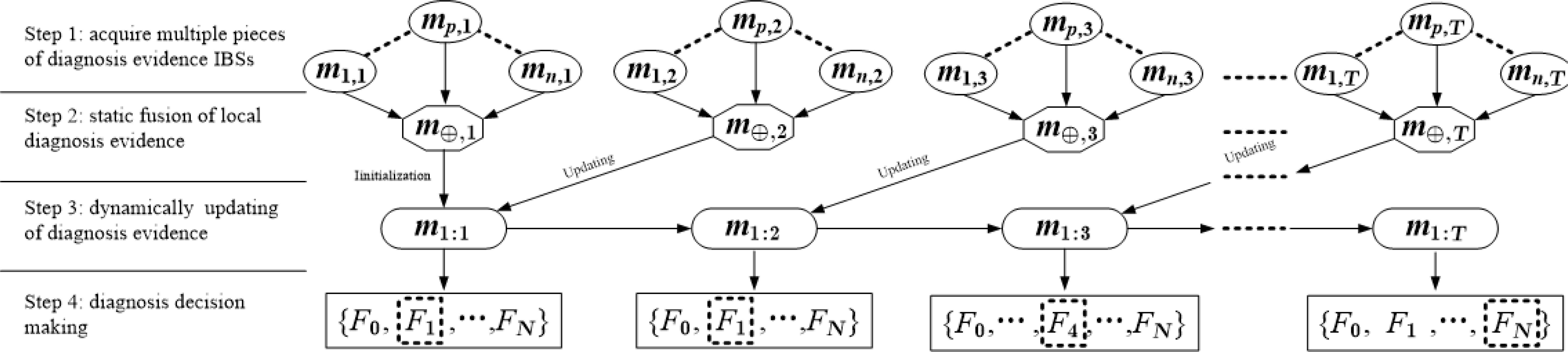
The diagnosis procedure based on the linear updating rule of IBSs
The whole procedure consists of 4 steps. Step 1 is to acquire n local pieces of diagnosis evidence at each step, denoted as mp,t, p=1,2,…,n, t=1,2,…,T. The intervals of belief masses in mp,t present the belief degrees that on-line monitoring information, given by the pth source at the tth step, supports each fault mode and the subset of fault modes in the frame of discernment Θ. mp,t can be given by the pattern matching methods12 or diagnosis experts17. Step 2 is to fuse n local pieces of diagnosis evidence. Since m1,t, m2,t,…, mn,t are simultaneously collected at the tth step, so the symmetric or static combination rule in Definition 3 is used to fuse them. The function of combination rule is to reduce the uncertainty of local diagnosis evidence such that the fused IBS m⊕,t is more certain and precise than any local IBS.
In the following updating step, m⊕,t is regarded as the incoming diagnosis evidence. The extended linear updating rule in Definition 8 is used to update the previous updated diagnosis evidence m1:t-1 with m⊕,t. As a result, the current global evidence m1:t can be recursively generated at each step, which contains the whole diagnosis information from the 1st step to the current step. At the 1st step, m1:t is initialized as m⊕,1, as we have not prior information to update. The last step is to make a diagnosis decision at the each step based on the global diagnosis evidence m1:t. There are two popular criterions which must be complied with in diagnosis decision: (1) for the determined fault proposition, the left and right endpoints of its belief mass interval are greater than those of any other fault propositions respectively; (2) The right endpoint of m(Θ) (complete ignorance) must be smaller than a certain threshold. It is set as 0.3 experientially.
4.3. The new methods for selecting linear combination weights
In the above step 3, we have to determine the linear combination weight {αt,βt} at each step when using the extended linear updating rule. In this section, we present two available strategies based on the similarity measure between two IBSs.
In Dempster-Shafer evidence theory, the evidence distance is the main way to quantify the dissimilarity between two belief structures (i.e.,BBAs or IBSs)29, so the concepts of distance and similarity are linked in an inverse way. That is to say, the lesser the distance between two IBSs, the greater their similarity22. Therefore, the similarity measure Sim(m1,m2) between m1 and m2 on the same frame of discernment Θ, can be obtained from the distance measure given in Definition 7 as
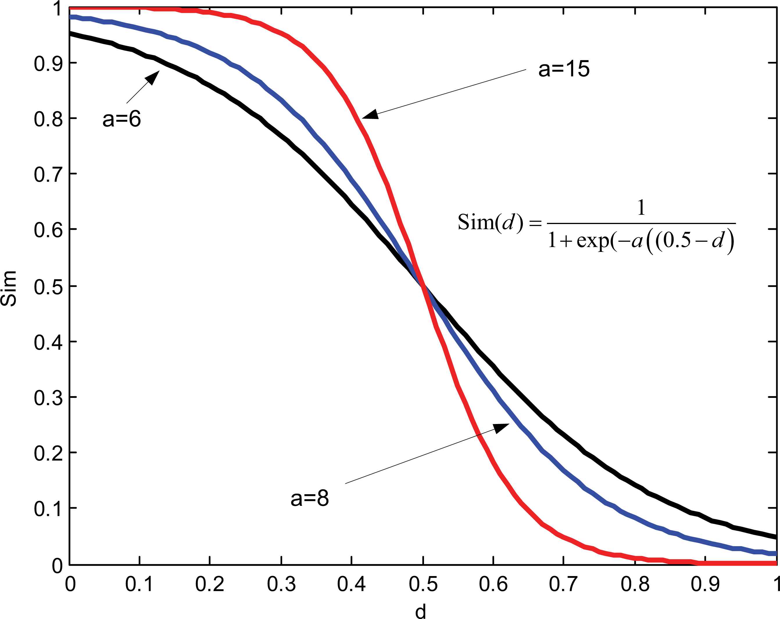
The relationship between dIBS and Sim with different a
It can be seen from the Fig.2 that Sim=0.5 when d =0.5, their similarity rapidly trends towards 0 when d increases from 0.5 to 1, their similarity rapidly trends towards 1 when d decreases from 0.5 to 0. In the existing definitions of similarity measure, the function f is usually endowed with the linear form, for example f =1-d 31. However, compared with the linear function, the sigmoid function can polarizes the similarity relationship between two IBSs, which is more beneficial to fault classification problem. Degree of polarization can be changed by adjusting a.
If there are N IBSs on Θ, as m1, m2,…, mN, then the degree that mi is supported by the other N-1 IBSs can be given as31
The credibility degree of mi is defined as 31
Obviously,
Actually, from the extended linear updating rule in Eqs.(15) and (16), it can be seen that the current updated evidence is the weighted sum of the historical updated evidence m1:t-1 and the current diagnosis evidence m⊕,t. The corresponding weights {αt,βt} determine the combining proportions of these two pieces of evidence respectively. Suppose the updated IBSs m1:t-2 and m1:t-1 at the (t-2)th and the (t-1)th steps have been recursively obtained respectively and the incoming fused IBS m⊕,t at the tth step and the next fused IBS m⊕,t+1 at the (t+1)th step have also been calculated respectively from step 2 in Fig.1. We present two available strategies for getting {αt,βt}.
The first is called the look-back based (LBB) updating strategy using similarity between m1:t-2, m1:t-1 and mt. Firstly, we calculate similarities between them by Eq. (18)
Secondly, we calculate the credibility degrees of m1:t-2, m1:t-1 and m⊕,t by Eq. (20)
According to the credibility degrees, we can set the linear combination weight at the tth step as
Obviously, the LBB assigns a higher weight αt to the historical diagnosis evidence m1:t-1 than βt to the current diagnosis evidence m⊕,t. Meanwhile, {αt,βt} are always adjusted dynamically with the changes of similarities between m1:t-2, m1:t-1 and m⊕,t. The LBB is derived from the kind of experts’ cognition that the historical diagnosis information is more reliable than the current diagnosis information.
The second is called the look-ahead based (LAB) updating strategy using similarity between m1:t-1, m⊕,t and m⊕,t+1. Repeating the above process, we can obtain Crd(m1:t-1), Crd(m⊕,t) and Crd(m⊕,t+1), and then set the linear combination weight at the tth step as
The LAB follows the other kind of experts’ cognition that one has to look ahead and behind before taking actions. It introduces the future diagnosis information mt+1 to updating by the smoothing factor Crd(m⊕,t+1), which can be used to adjust {αt,βt} dynamically according to the changes of similarities between m1:t-1, m⊕,t and m⊕,t+1. More specifically, Sim(m1:t-1,m⊕,t+1)> Sim(m⊕,t,m⊕,t+1) means that the belief mass distribution of m⊕,t is distinctly different from that of m1:t-1 and m⊕,t+1. Since there is commonly a reciprocal causation relation among running states of equipment at adjacent time steps, so this conflict between m1:t-1 and m⊕,t is likely caused by the uncertain disturbances at the tth step. Therefore, m1:t-1 is more reliable than m⊕,t, Crd(m⊕,t+1) is assigned to αt such that the former has bigger combining proportion than the latter. Moreover, since m1:t-1 includes all of the historical information by iterative updating process, so although Sim(m1:t-1,m⊕,t+1)=Sim(m⊕,t,m⊕,t+1), Crd(m⊕,t+1) is still assign to αt. On the other hand, Sim(m1:t-1,m⊕,t+1)<Sim(m⊕,t,m⊕,t+1) means that running states of equipment have significant change, the new state continues for adjacent two steps. In this case, Crd(m⊕,t+1) is assign to βt so as to reduce the inertia of the historical information.
As a result, the LBB and LAB have the different scope of application. In the following typical fault experiments, their functions and performance will be compared and analyzed in detail.
5. The static reliability and dynamic sensitivity indices for diagnosis
In order to assess the performance of updating diagnosis algorithms, we design the static reliability index (SRI) and dynamic sensitivity index (DSI).
Let us denote the FoD as Θ={F0, F1,…, FN}. Suppose that the length of a diagnosis period is T time steps and the equipment being monitored goes through totally M states from FT1 to FTM, FTi ∈ Θ (i=1,2,…M) in this period.
SRI can be defined as
Correspondingly, the DSI can be defined as
It emphasizes that the contribution of
6. Experiments
6.1. Experiment settings
In this paper, we choose the ZHS-2 machine rotor system as shown in Fig.3 to test the proposed linear updating algorithms with the different strategies of selecting linear combination weights {αt,βt} The typical faults seeded in the system are motor bracket loosening (F1), rotor misalignment (F2) and rotor unbalance (F3) 1,12. As one goal of fault diagnosis, we also add F0 as the normal state of the system. Therefore, the frame of discernment can be described as Θ = {F0, F1, F2, F3}.
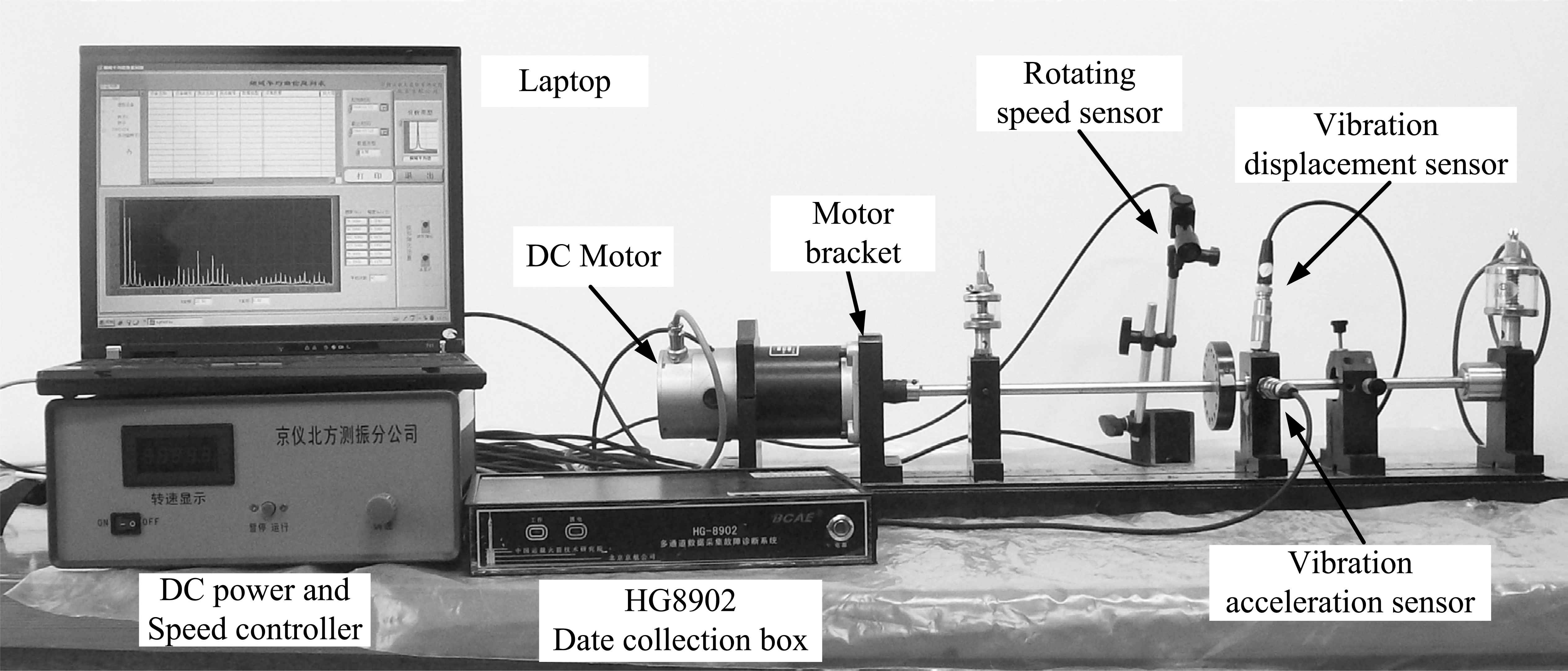
ZHS-2 machine rotor system
A vibration displacement sensor and a vibration acceleration sensor are installed on the bracket of rotor respectively in order to collect vibration signals in both vertical and horizontal directions. The collected vibration signals are inputted into HG-8902 data collector, and then processed by signal conditioning circuits. Finally, the processed signals are inputted into a laptop. The fault features can be extracted from these signals by HG-8902 data analysis software under the environment of Labview. The amplitudes of fundamental, double, triple vibration acceleration frequencies (denoted as f×1~ f×3 respectively for short) and average amplitude of vibration displacement (denoted as da for short) are selected as fault feature parameters 1,12.
6.2. Experiment results
We conduct four typical fault experiments usually happened in real world, on which, the proposed LBB(look-back based) and LAB(look-ahead based) strategies for selecting {αt,βt} are compared with the basic strategies IIB(infinite inertia based), ZIB(zero inertia based) and PIB (proportional inertia based). Moreover, in these experiments, we also use the Dempster’s combination rule of IBSs (DCR) in Definition 3 to obtain the updated results, namely, m1:t=m⊕,1 ⊕ m⊕,2⊕ … ⊕ m⊕,t. From the comparison between DCR and the liner updating rule, it can be seen that static/symmetric DCR may be no longer suitable for evidence updating, especially when system states change over time.
Experiment 1:
The rotor system always stably keeps in normal state at the tth step, t=1,2,…,10, the time interval between two steps Δt = 16s.
According to the diagnosis procedure in Fig.1, at each time step, the method in Ref.12 is used to get the four local IBSs respectively from the monitoring data of f×1, f×1, f×3 and da, and then, the static combination rule in Definition 3 is used to fuse the local IBSs to obtain the incoming diagnosis evidence (IDE) m⊕,t as shown in Table 4. Fig.4 shows the updated results obtained recursively using the linear updating rule with LBB, LAB, IIB, ZIB, PIB and DCR. Here, m⊕,t({F0}), m⊕,t({F1}), m⊕,t({F2}) and m⊕,t({F3}) are also shown in Fig 4 except m⊕,t (Θ), because m⊕,t (Θ) usually becomes relatively small by optimal combination such that it rarely influences the following decision making. For example, the interval value of belief masses of m8 illustrated in Fig.4.
The updated IBSs of LBB, LAB, IIB, ZIB, PIB and DCR in experiment 1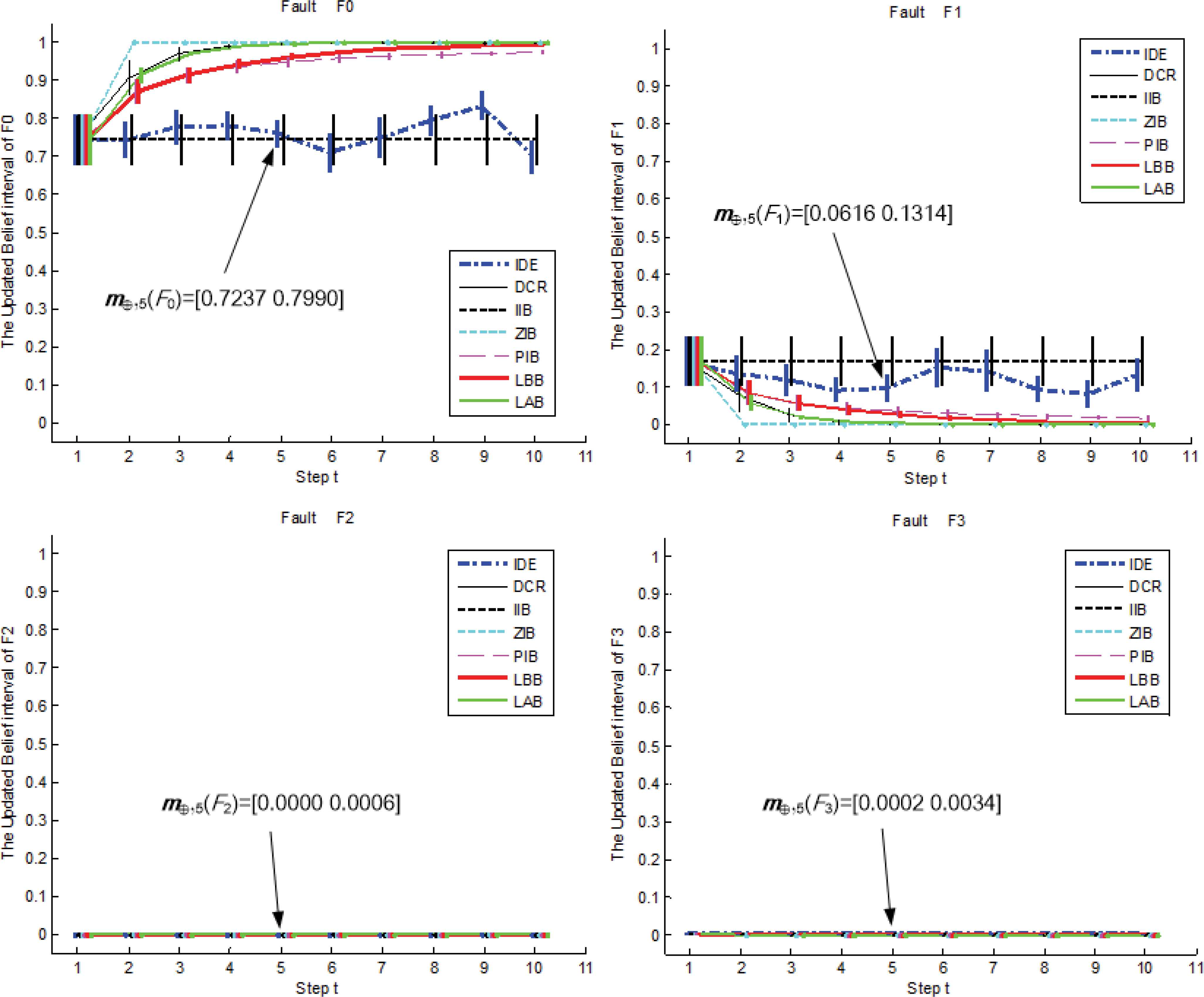
| t | m⊕,t{F0} | m⊕,t{F1} | m⊕,t{F2} | m⊕,t{F3} | m⊕,t (Θ) |
|---|---|---|---|---|---|
| 1 | [0.6792 0.8103] | [0.1023 0.2344] | [0.0000 0.0001] | [0.0004 0.0052] | [0.0639 0.1136] |
| 2 | [0.6935 0.7922] | [0.0861 0.1846] | [0.0000 0.0005] | [0.0003 0.0046] | [0.0968 0.1487] |
| 3 | [0.7312 0.8230] | [0.0747 0.1619] | [0.0000 0.0002] | [0.0002 0.0029] | [0.0827 0.1296] |
| 4 | [0.7437 0.8186] | [0.0564 0.1256] | [0.0000 0.0006] | [0.0003 0.0046] | [0.1048 0.1509] |
| 5 | [0.7237 0.7990] | [0.0616 0.1314] | [0.0000 0.0006] | [0.0002 0.0034] | [0.1182 0.1674] |
| 6 | [0.6595 0.7609] | [0.1001 0.2033] | [0.0000 0.0005] | [0.0002 0.0031] | [0.1112 0.1685] |
| 7 | [0.6930 0.8029] | [0.0876 0.1977] | [0.0000 0.0004] | [0.0005 0.0066] | [0.0843 0.1350] |
| 8 | [0.7548 0.8317] | [0.0571 0.1271] | [0.0000 0.0002] | [0.0003 0.0039] | [0.0928 0.1376] |
| 9 | [0.7947 0.8713] | [0.0456 0.1153] | [0.0000 0.0002] | [0.0006 0.0073] | [0.0668 0.1038] |
| 10 | [0.6559 0.7439] | [0.0879 0.1768] | [0.0000 0.0014] | [0.0002 0.0030] | [0.1395 0.1977] |
The incoming diagnosis evidence (IDS) m⊕,t
Table 5 lists the static reliability index (SRI) and dynamic sensitivity index (DSI) of the updated results in descending order. In our experiments, the parameter a of similarity measure is set as 8.
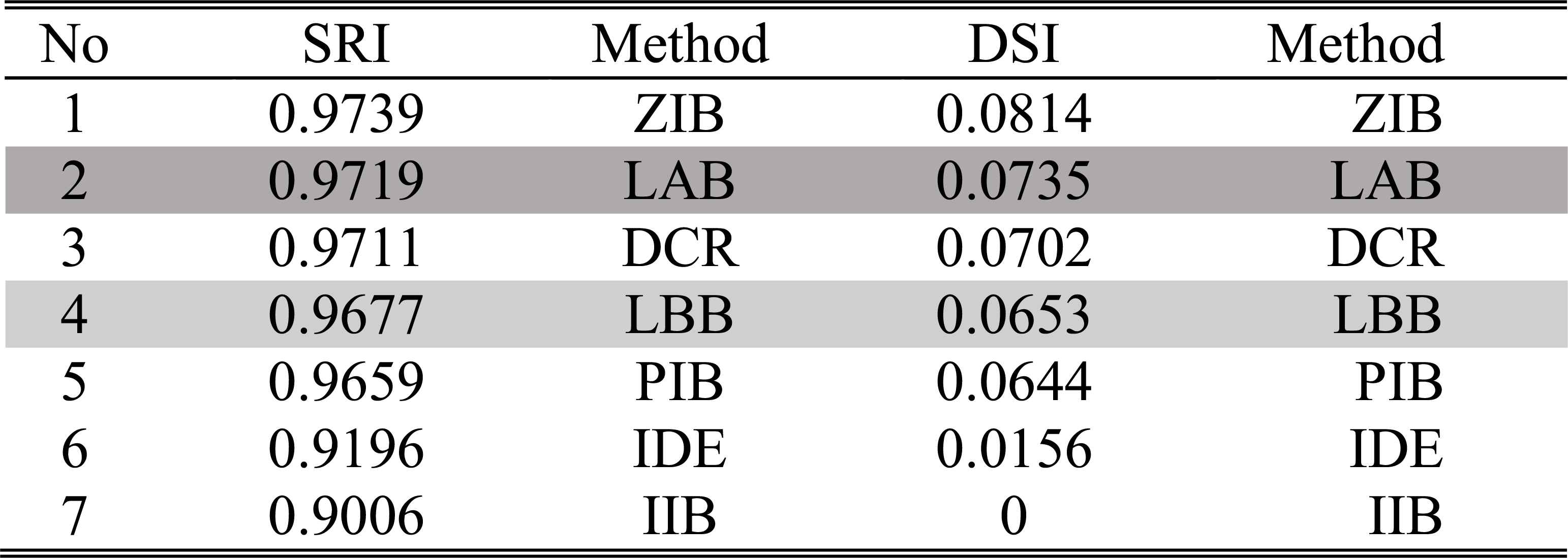
The ordering of SRIs and DSIs of different methods in experiment 1
It can be seen that from Table 5 that the performance indices of the other updating algorithms except the IIB, are all better than the IDE’s. That is to say, although the diagnosis decisions made from all the methods are correct (F0 happens), the dynamic updating procedure can provide more reliable diagnosis results than the static fusing procedure. In the IIB, {αt,βt}={1,0}, it means that m1:t = m1:t-1 according to the extended linear updating rule in Eqs. (15) and (16). Since m1:1= m⊕,1, the updated result at each step is always taken as m⊕,1, therefore, the IIB is quite insensitive to the change of the incoming diagnosis evidence. In the PIB, when t=1, {αt,βt} = {1,0}, otherwise, {αt,βt}={(t-1)/t,1/t}. In the ZIB, {αt,βt}={0,1}, so its m1:t is completely determined by the m⊕,t, and since m⊕,t({F0}) is always larger than m⊕,t({F1}), m⊕,t({F2}), m⊕,t({F3}) and m⊕,t(Θ), according to the extended linear updating rule, m1:t({F0}) can immediately converge to [1,1] at the 2nd step and is unchanged until the last step. Therefore, in this experiment, the ZIB have the best performance on reliability and sensitivity. As m⊕,t always supports F0, so the DCR also makes belief masses converge to F0. Although the LAB and LBB do not provide better results than the ZIB, both of them are available in accordance with the decision criterions in Fig.1.
Experiment 2:
The rotor system encounters abrupt external disturbances at different time steps, and then returns to its normal working condition when the disturbances disappear. There are three detailed cases.
Case 1: The system only encounters the disturbance at the 6th step. It causes the false fault “motor bracket loosening (F1)”.
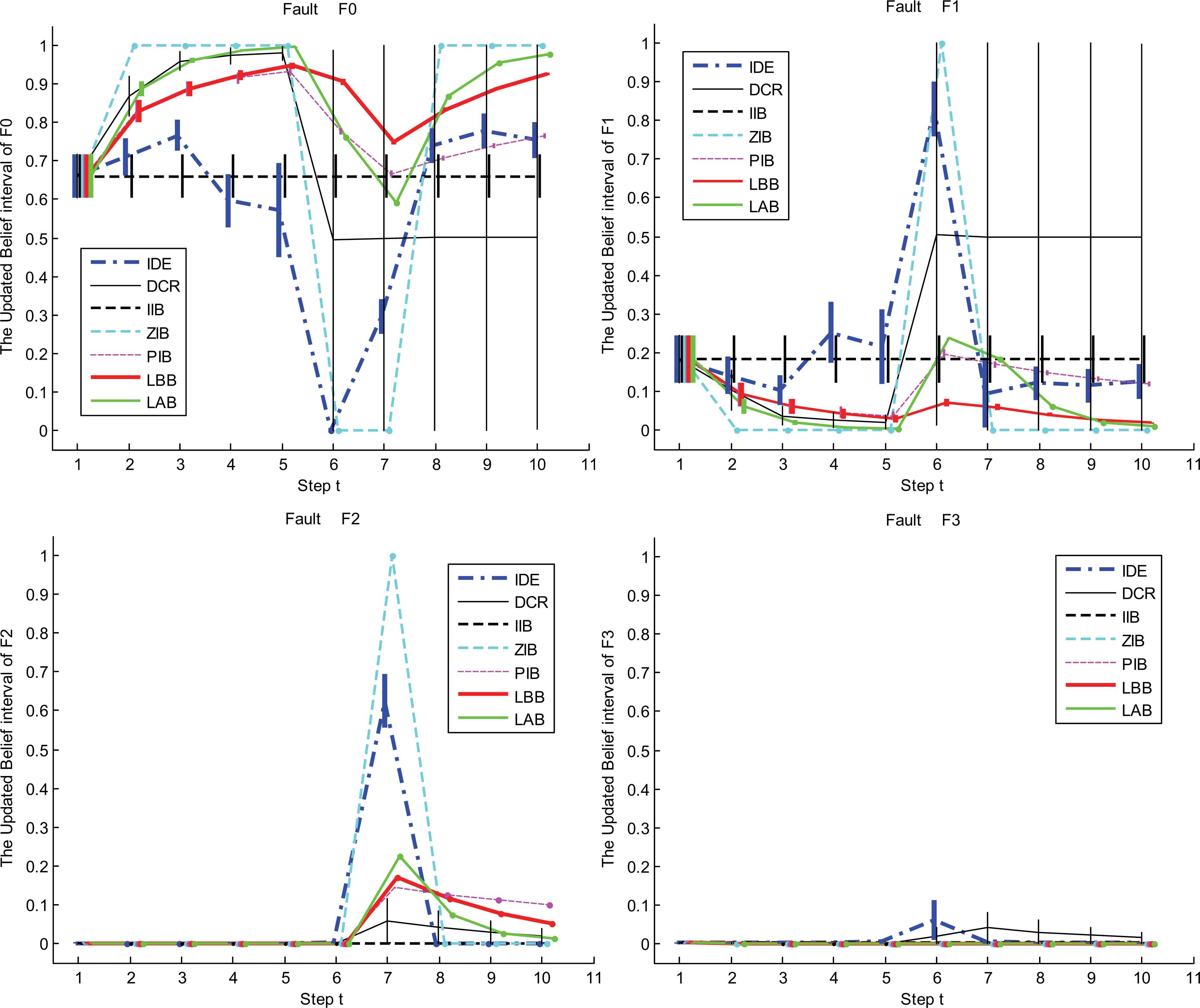
Case 2: The system continuously encounters the disturbances at the 6th and 7th steps. They cause the false faults “motor bracket loosening (F1)” and “rotor misalignment (F2)” respectively.
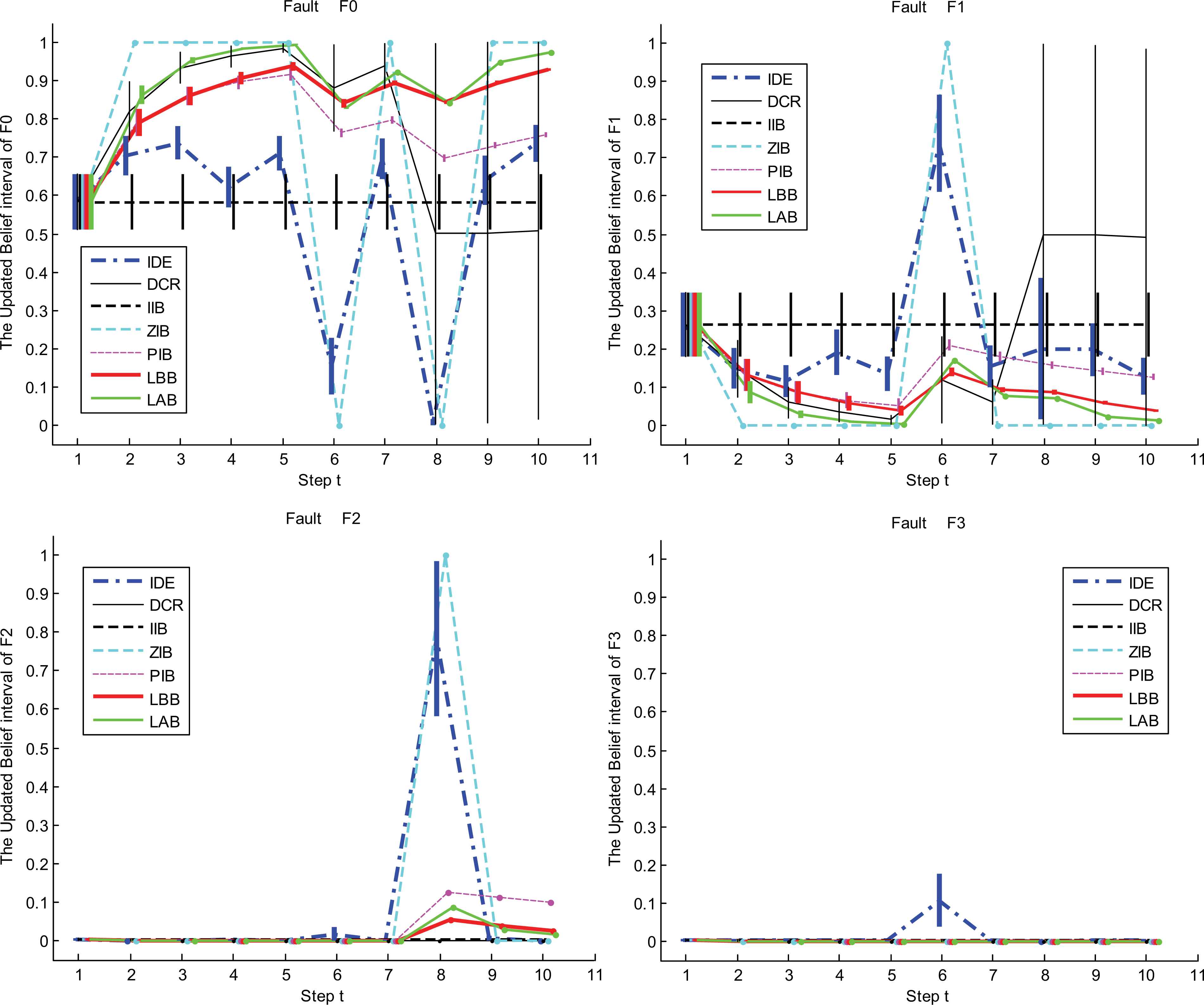
Case 3: The system intermittently encounters the disturbances at the 6th and 8th steps respectively. They cause the false faults “motor bracket loosening (F1)” and “rotor misalignment (F2)” respectively.
The updated results in three cases are shown in Fig.5, Fig.6 and Fig.7 respectively. An ideal diagnosis system should be immune to the disturbances. It can be concluded from these three figures that, the disturbances are so strong that the incoming diagnosis evidence (IDE) incorrectly support false faults. The disturbances even cause that the DSIs of IDE are negative. For example, Table 6 lists the changes of similarity
The updated IBSs of LBB, LAB, IIB, ZIB, PIB and DCR in case 1 of experiment 2 The updated IBSs of LBB, LAB, IIB, ZIB, PIB and DCR in case 2 of experiment 2 The updated IBSs of LBB, LAB, IIB, ZIB, PIB and DCR in case 3 of experiment 2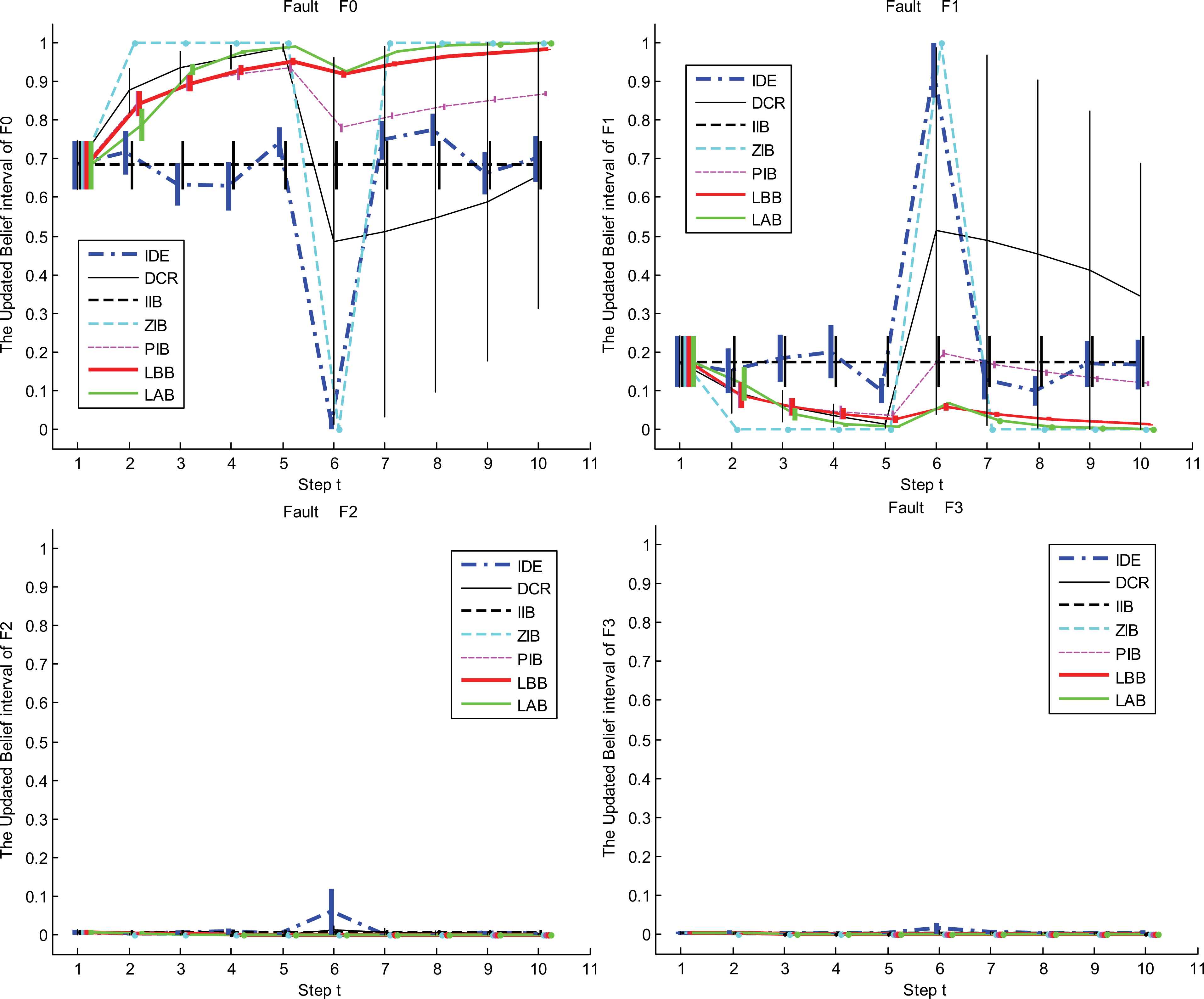
| FT | t | Sim |
|
|
|---|---|---|---|---|
| F0 | 1 | 0.8586 | - | - |
| 2 | 0.8990 | 0.0404 | 1 | |
| 3 | 0.9288 | 0.0298 | 1/2 | |
| 4 | 0.7819 | −0.1469 | 1/3 | |
| 5 | 0.7688 | −0.0131 | 1/4 | |
| 6 | 0.0324 | −0.7364 | 1/5 | |
| 7 | 0.1976 | 0.1653 | 1/6 | |
| 8 | 0.9152 | 0.7175 | 1/7 | |
| 9 | 0.9290 | 0.0138 | 1/8 | |
| 10 | 0.9195 | −0.0095 | 1/9 |
The similarity changes of IDE in case 2
From Table 6, we can get DSI=-0.0135, SRI=0.7231 according to Eqs. (31) and (30). In the same way, we can calculate the SRI and DSI of each method in three cases as shown in Table 7, Table 8 and Table 9 respectively.
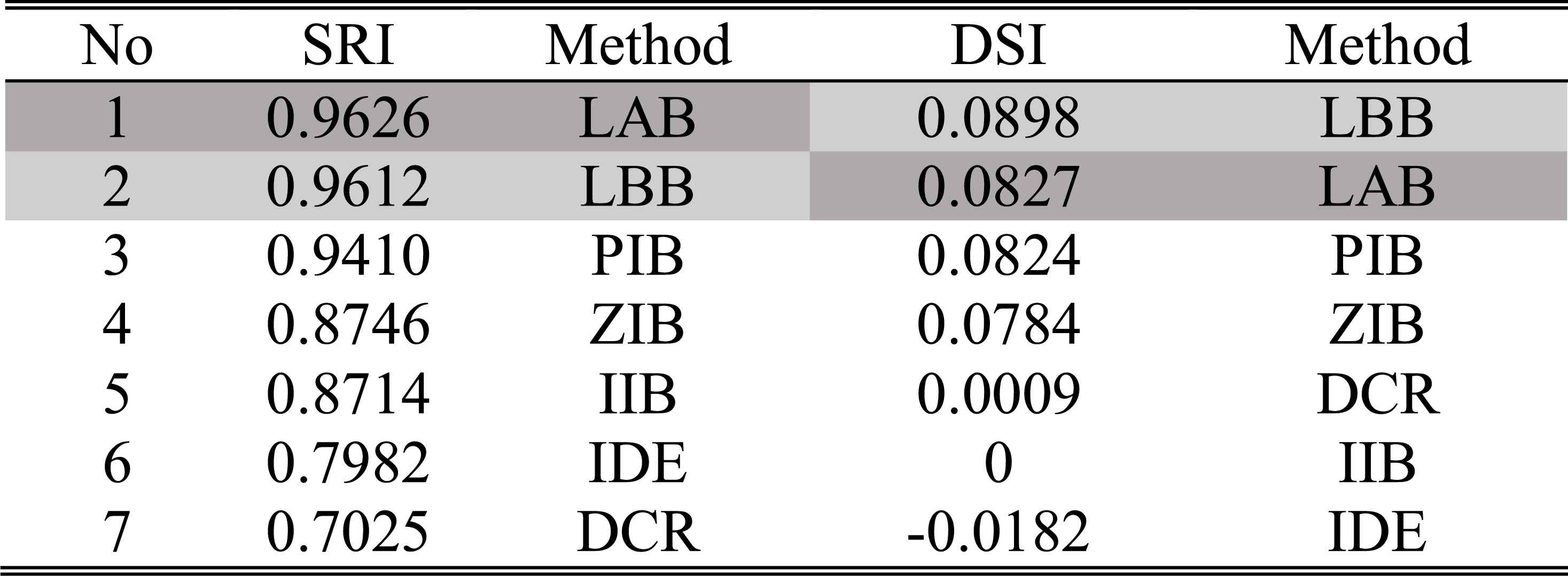
The ordering of SRIs and DSIs of different methods in case 1 of experiment 2
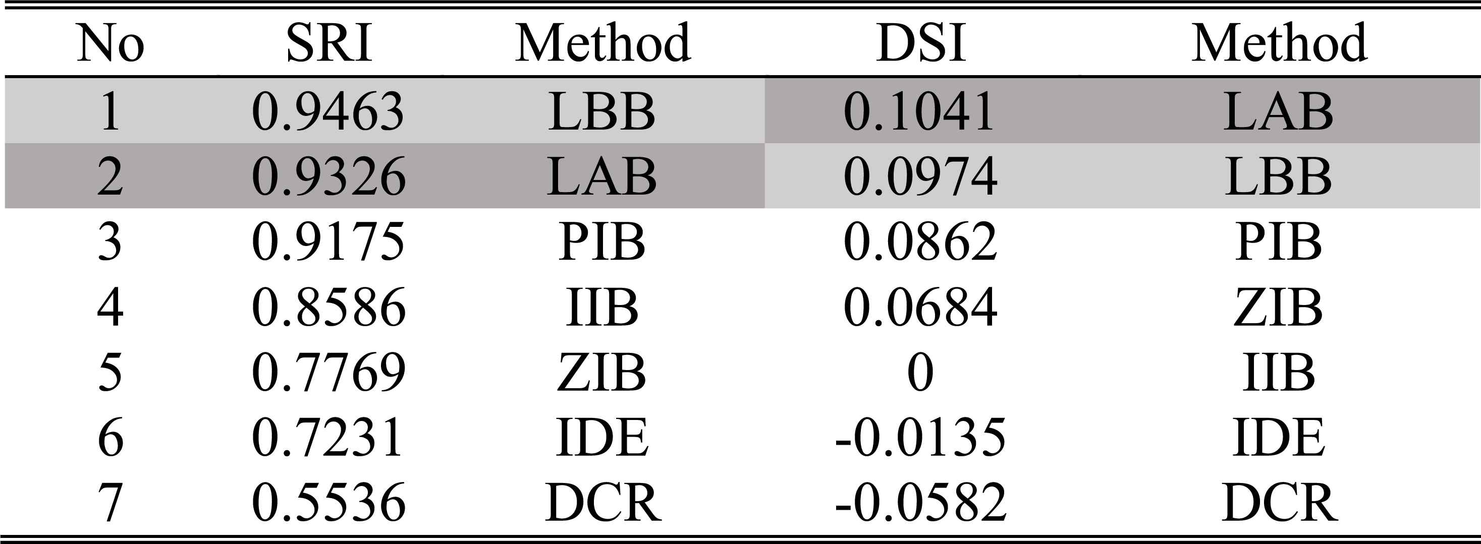
The ordering of SRIs and DSIs of different methods in case 2 of experiment 2
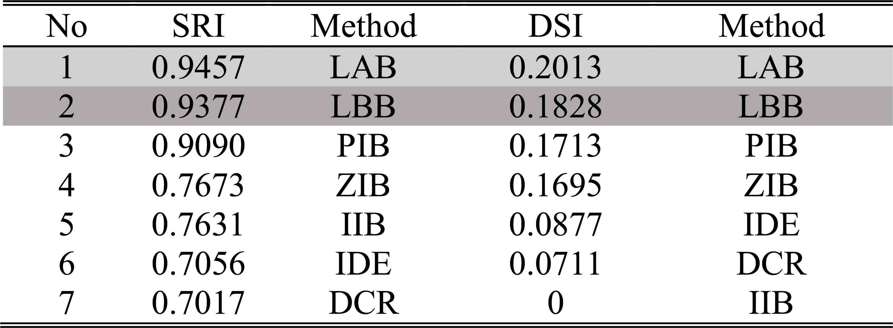
The ordering of SRIs and DSIs of different methods in case 3 of experiment 2
It can be seen from these figures and tables that the evidence updating strategies in LAB, LBB, PIB and IIB all make the correct judgment according to the decision criterions. Obviously, the static and dynamic performance of the LAB and LBB are superior to that of the other methods. When the disturbances happen, the judgments given by the ZIB are always utterly wrong, because it adopts the extreme strategy to support the incoming evidence and ignore the inertia of historical evidence. On account of the conflicts between the incoming diagnosis evidence, since the 6th step, the interval widths of belief masses given by the DCR become too large to make decisions. So, in these cases, the DCR is no longer applicable.
Experiment 3:
The rotor system goes through the intermediate stage between normal and fault. More specifically, the system is normal from the 1st step to the 5rd step, from the 6th step to the 7th step, the running status of the system gradually degrades to “motor bracket loosening (F1)”, and then, F1 really happens at remaining three steps.
Fig.8 shows the updated results and Table 10 lists the corresponding performance indices. Contrary to what we have observed in the above experiments, the ZIB, in this experiment, returns to the best performance just as illustrated in experiment 1. But, distinctly, in the face of the different changes of the system states, the performance of the ZIB fluctuates and becomes unstable. The DCR is still inapplicable because of the same reason as in experiment 2. The IIB only relies on the historical evidence, and completely ignores the change of the system states from F0 to F1. In the PIB, {αt,βt} = {t/(t+1),1/(t+1)}, when t increases, βt tends to 0, so the share of the incoming evidence in the updated result will be smaller and smaller. It leads to the slow speed of converging to the new state F1 and bad decisions. On the contrary, the LAB still keeps good behaviors. The LBB can be interpreted as the tradeoff between the LAB and PIB.
The updated IBSs of LBB, LAB, IIB, ZIB, PIB and DCR in experiment 3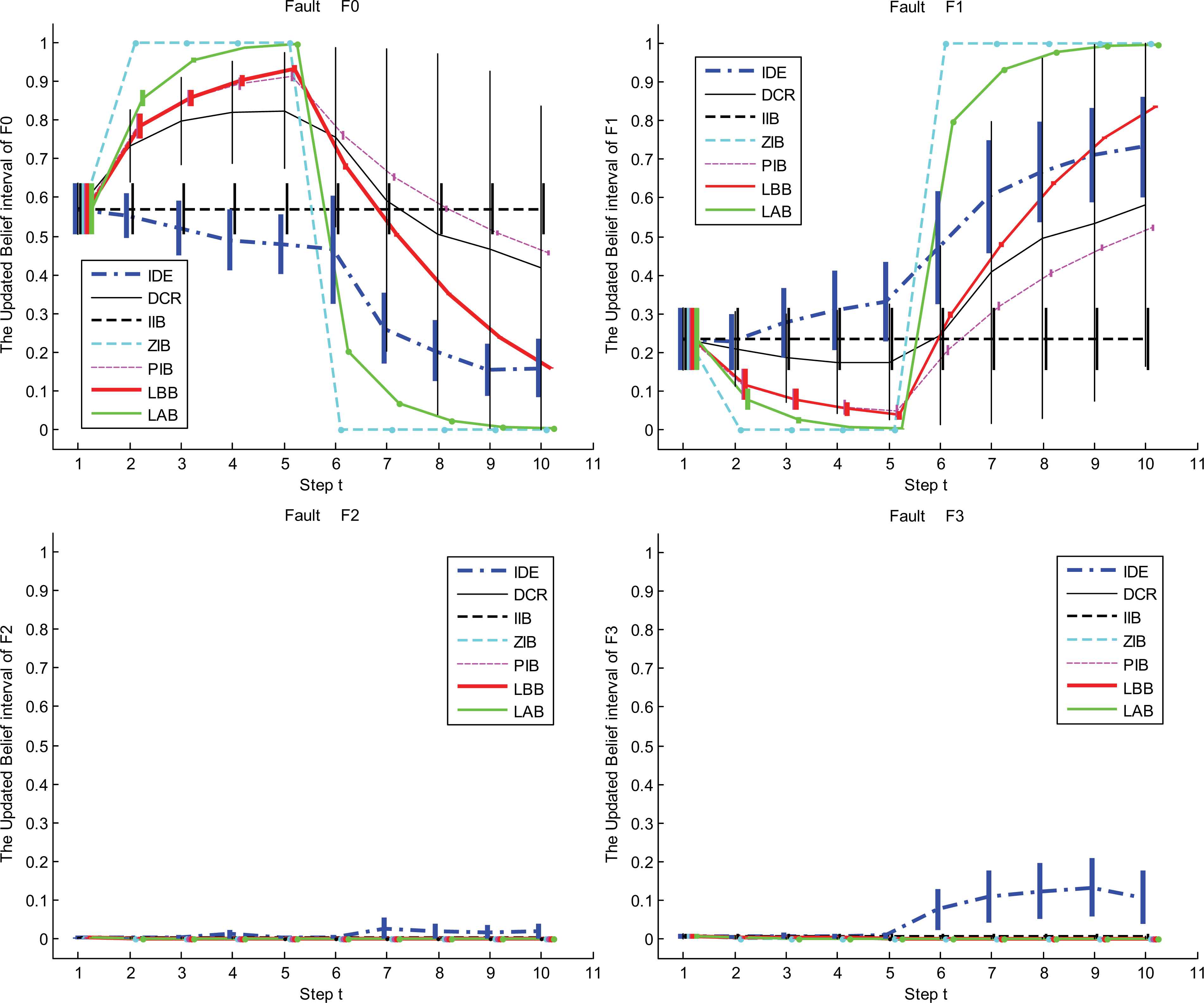
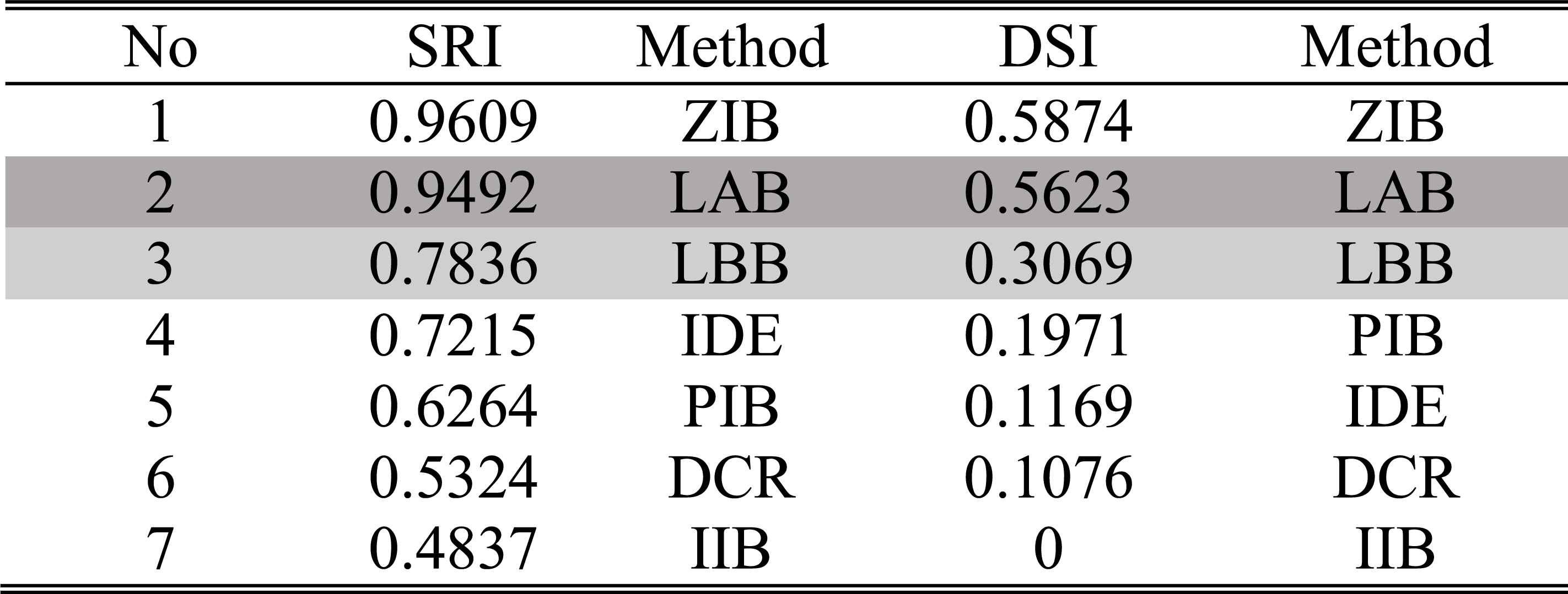
The ordering of SRIs and DSIs of different methods in experiment 3
Experiment 4:
The rotor system is normal from the 1st step to the 5th step, but the fault “motor bracket loosening (F1)” suddenly happens at the 6th step and goes on until the 10th step.
Fig.9 shows the updated results and Table 11 lists the corresponding performance indices. The performance of each method is similar with that in experiment 3. Obviously, compared with other methods, the performance of the LAB keeps stable.
The updated IBSs of LBB, LAB, IIB, ZIB, PIB and DCR in experiment 4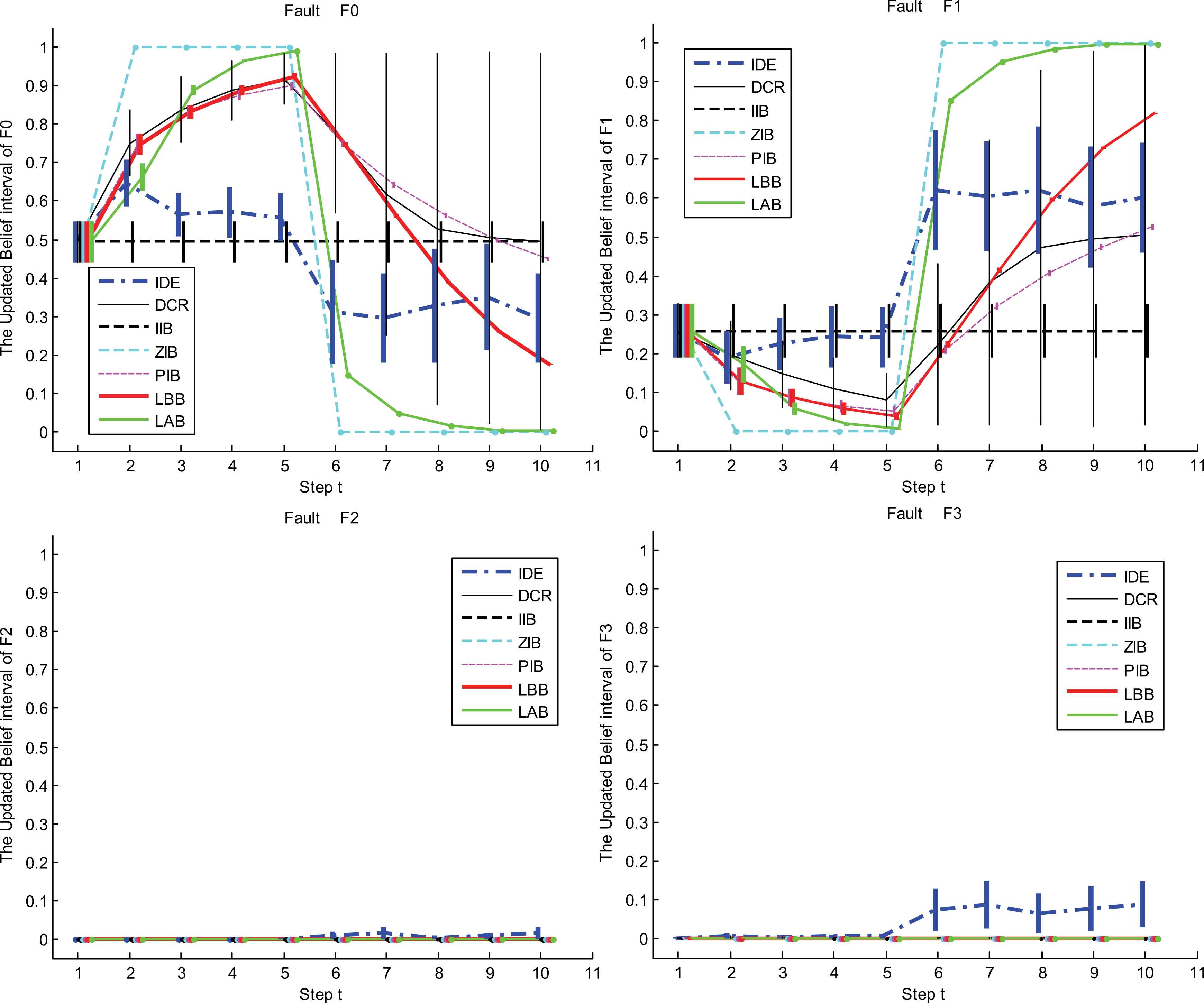
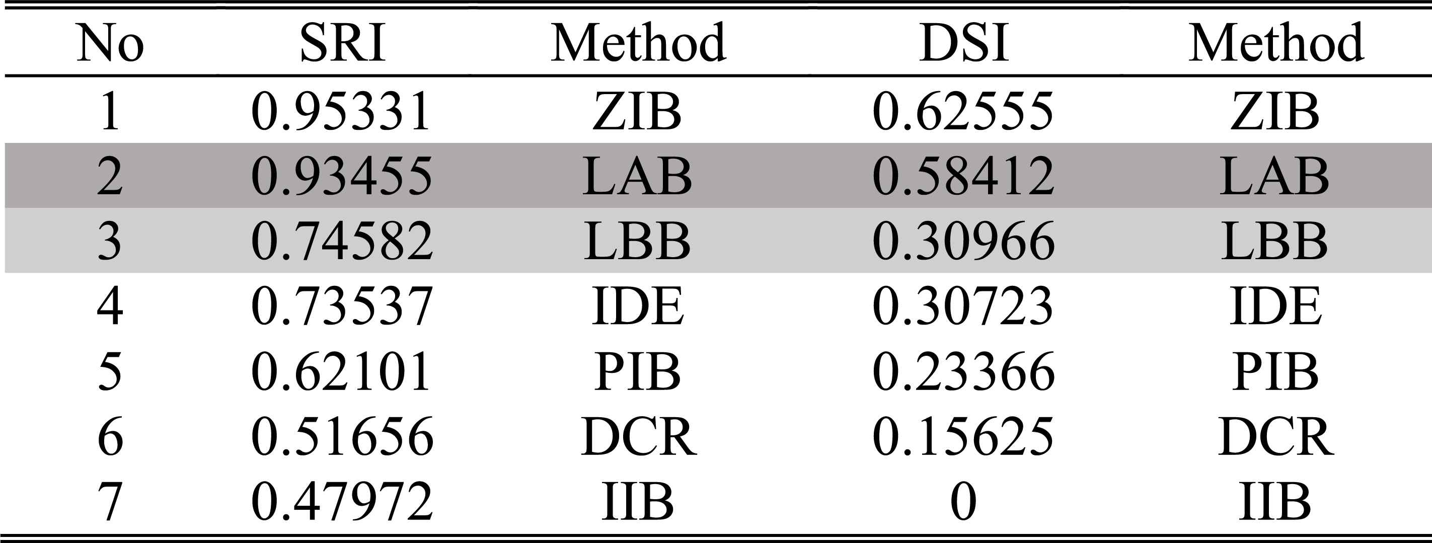
The ordering of SRIs and DSIs of different methods in experiment 4
Furthermore, we give the average value of performance indices of every method in three experiments as shown in Table 12.
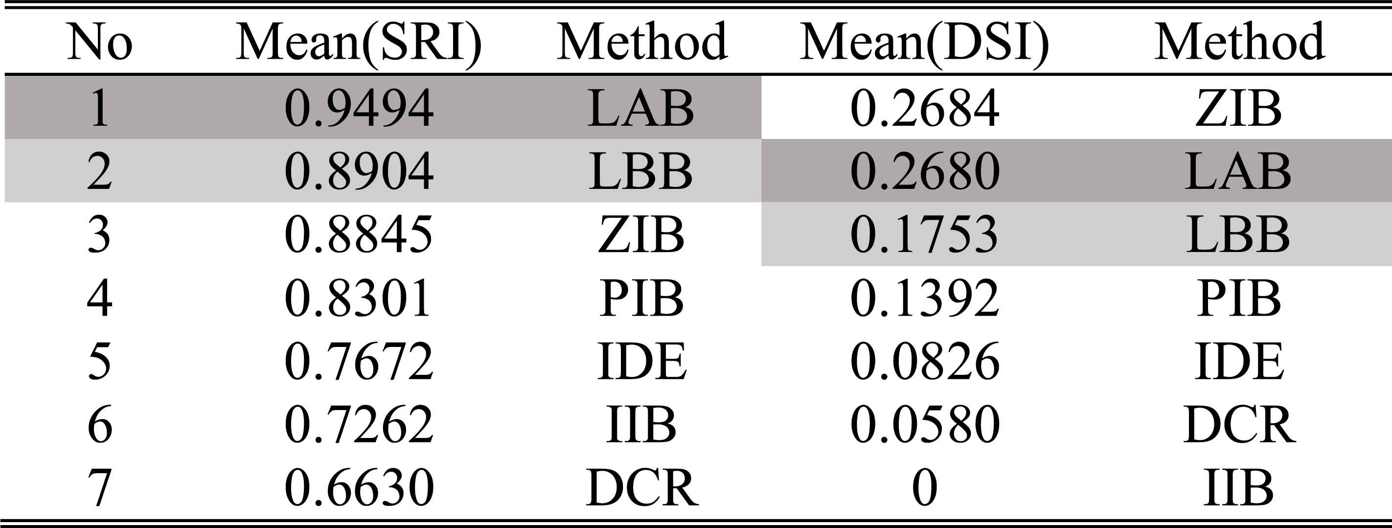
The ordering of average values of SRI and DSI in four experiments
It can be seen from this table that the LAB have the best comprehensive performance. Although the dynamic sensitivity of the ZIB is the same with that of the LAB, the absolutely wrong judgments that it makes in experiment 2 lead to the low static reliability. The IIB and DCR are almost inapplicable to dynamic diagnosis because they rarely adapt to the different changes of system states. In summary, the proposed LAB and LBB can deal with the typical changes of system states. Specifically speaking, in the initial operation stages, the monitored system is commonly stable and healthy. In this case, the LBB can be used to avoid some false-alarms caused by the intermittent or abrupt external disturbances as shown in experiment 2. With the increasing of the running time, if the reliability of system deteriorates, the LAB can respond to the disturbances and the abrupt or gradual faults rapidly and accurately shown in the last three experiments.
7. Conclusion
In this paper, a novel idea of evidence updating is introduced into dynamic/on-line fault diagnosis. Based on interval-valued belief structures, the new updating strategies for dynamic fault diagnosis are presented. The main contributions of the paper include: (1) The classical linear updating rule are extended to the framework of IBSs, which can be used to recursively fuse the “dissymmetric” and “dynamic” diagnosis evidence over time; (2) The LAB and LBB method can adaptively adjust the linear combination weights according to the similarity relationship between the incoming diagnosis evidence and the previous diagnosis evidence; (3)The static reliability and the dynamic sensitivity indices are designed to evaluate the performance of an updating strategy. (4) Finally, the typical fault experiments of machine rotor show the effectiveness of the proposed updating strategies.
The presented methods could be further investigated in several ways. First of all, the distance between two interval-valued structures is a basic tool for assessing the performance of IBSs-based classification algorithms. From the perspective of interval mathematics or interval computations32–33, the distance between two interval-valued structures is actually the distance between two interval-valued vectors, in this case, the value of distance should be also an interval value, not be a point value as given in Definition 7 such that IBS can manifest its advantage of impreciseness control over BBA. Therefore, we can further consider the other alternative distances with interval values by using some interval metrics as given in Refs.32–33; Second, when prior diagnosis information is available, one can introduce on-line learning algorithm to optimize the parameter a in the similarity measure such that the updating procedure adapts to the changes of system state. Third, the evidence updating strategy should be easily applicable to other fields such as dynamic target recognition and expert systems but it needs to be validated by experimental studies or real world applications.
Acknowledgements
This work was supported by the NSFC (No. 61374123, 61433001, 61573076, 61573275), the Zhejiang Open Foundation of the Most Important Subjects and the Zhejiang Province Research Program Project of Commonweal Technology Application (No. 2016C31071)
Appendix A.
Proof of Lemma 1
Proof. Let m1=([a1-,a1+],[a2-,a2+],…[aN-,aN+]), m2=([b1-,b1+],[b2-,b2+],…[bN-,bN+]), m3= ([c1-,c1+], [c2-,c2+],…[cN-,cN+]) be three interval-valued vectors in Ω, also be three IBSs on the same frame of discernment Θ. By the use of Eqs. (8) and (9), their corresponding Pignistic probability functions can be calculated as
Then, IBetPm1, IBetPm2 and IBetPm3 are three interval-valued vectors in space Ω′. We must check that d in Definition 7 satisfies four axioms for (Ω′, dIBetP) to be a metric space for any IBetPm1, IBetPm2, IBetPm3 ∈ Ω′:
- M1:
Nonegativity: d(IBetPm1, IBetPm2) ≥ 0;
- M2:
Nondegeneracy: d(IBetPm1,IBetPm2)=0 ⇔ IBetPm1 = IBetPm2;
- M3:
Symmetry: d(IBetPm1, IBetPm2)=d(IBetPm2, IBetPm1);
- M4:
Triangle inequality: d(IBetPm1, IBetPm2) ≤ d(IBetPm1, IBetPm3) + d(IBetPm3, IBetPm2), ∀IBetPm3 ∈ Ω′.
Since
Axiom M3 is obvious as
Finally, let’s prove axiom M 4,
References
Cite this article
TY  - JOUR
AU  - Xiaobin Xu
AU  - Zhen Zhang
AU  - Dongling Xu
AU  - Yuwang Chen
PY  - 2016
DA  - 2016/06/01
TI  - Interval-valued Evidence Updating with Reliability and Sensitivity Analysis for Fault Diagnosis
JO  - International Journal of Computational Intelligence Systems
SP  - 396
EP  - 415
VL  - 9
IS  - 3
SN  - 1875-6883
UR  - https://doi.org/10.1080/18756891.2016.1175808
DO  - 10.1080/18756891.2016.1175808
ID  - Xu2016
ER  -