
Semi-Supervised Density Peaks Clustering Based on Constraint Projection
- DOI
- 10.2991/ijcis.d.201102.002How to use a DOI?
- Keywords
- Semi-supervised learning; Density peaks clustering; Pairwise constraint; Constraint projection
- Abstract
Clustering by fast searching and finding density peaks (DPC) method can rapidly identify the centers of clusters which have relatively high densities and high distances according to a decision graph. Various methods have been introduced to extend the DPC model over the past five years. DPC was originally presented as an unsupervised learning algorithm, and the thought of adding some prior information to DPC emerges as an alternative approach for improving its performance. It is extravagant to collect labeled data in real applications, and annotation of class labels is a nontrivial work, while pairwise constraint information is easier to get. Furthermore, the class label information can be converted into pairwise constraint information. Thus, we can take full advantage of pairwise constraints (or prior information) as much as possible. So this paper presents a new semi-supervised density peaks clustering algorithm (SSDPC) that uses constraint projection, which is flexible in loosening a few constraints over the learning stage. In the first stage, instances involving instance-level constraints and the remaining instances are concurrently projected to a lower dimensional data space led by the pairwise constraints, where viewing the distribution of data instances more clearly is available. Subsequently, traditional DPC is executed on the new lower dimensional dataset. Lastly, a few datasets from the Microsoft Research Asia Multimedia (MSRA-MM) image and UCI machine learning repository datasets are adopted in the experimental validation. The experimental results demonstrate that the proposed SSDPC achieves better performance than other three semi-supervised clustering algorithms.
- Copyright
- © 2021 The Authors. Published by Atlantis Press B.V.
- Open Access
- This is an open access article distributed under the CC BY-NC 4.0 license (http://creativecommons.org/licenses/by-nc/4.0/).
1. INTRODUCTION
The swift advancement in information technology has caused a massive increase in the amount of data generated. As storage becomes more affordable, we will continue to witness rapid growth. How much of this data makes sense to a naive user remains a challenge to researchers in fields such as data mining. As much of the data is not labeled, annotated, or captioned. One tool that has been used by the research communities to attempt to organize such mixed data is clustering. Clustering is grouping of objects into classes according to objects' similarities [1]. These classes exhibit close intra-class similarity and wide interclass difference, and much of this process is performed in an unsupervised way [2], where clustering in its original form takes mixed data that is unlabeled and attempts to categorize it [3].
Clustering is a useful technique because when datasets are apportioned into groups based on data homogeneity, we can hence give labels to such small groups. The process can adapt to changes and classify groups using suitable features [1]. Features describing each object are all the algorithm has available to separate the objects. Clustering can pinpoint sparse and dense areas in object space, and we can easily observe the entire distribution shapes and find any correlations in data marks. It can also be a preprocessing input to other algorithms, like classification and feature subset selection, which can conveniently work on the identified groups.
The most common approach in the use of clustering algorithms is with unlabeled data and without a tutor; it is therefore unsupervised. The input is simply a collection of data instances to be clustered based on some conceptual relationship. Unsupervised clustering can be greatly improved by some supervision, and numerous algorithms have been recommended to enhance the quality of clustering by employing supervision.
The clustering algorithms are not given any information at all, yet the experimenter in the real-world application domain may have some clues regarding the dataset that could be useful to the algorithm, for example, where to place each instance within the partition. Traditional unsupervised clustering algorithms cannot benefit from such information when it does exit [2]. We therefore are interested in clustering that requires some minimal involvement by the users and we refer to it as semi-supervised clustering.
Such supervision could be to place constraints either to revise the cost function or to master the distance and similarity measures [4]. This type of supervision is generally known as semi-supervised learning, it involves acquiring knowledge from labeled and at the same time unlabeled data by computers and natural systems like human beings [5–7]. This method is better than unsupervised and supervised learning as long as it offers improved performance and accuracy [5]. The system of semi-supervised learning works both for classification and clustering [8], hence the capability of unsupervised clusters can improve with little amounts of supervision by way of labels on the data or constraints [2]. Studies on semi-supervised clustering show that it is much more effective than unsupervised classification techniques [9–13].
Semi-supervised learning has been researched under models such as graph-based methods, mixture models, self-training, multi-view learning and co-training. The recent algorithms of semi-supervised clustering generalizes to two types: constraint and distance based. Constraint-based processes operated by users providing labels or constraints to control the algorithms to even more correct data separation [4,14]. This is achieved by tuning the objective function for gauging clustering such that it satisfies the constraints [4,15]. The constraints can be enforced through the clustering steps [2], or the clustering can be initialized and then constrained based on labeled examples [16]. Constraint-based semi-supervised clustering could, for example, use pairwise constraints, where two instances are grouped in the same or different bundles [4].
Pairwise constraint is a type of supervision information that specifies whether two instances of data locate in the same group (a must-link [ML]) or separate groups (a cannot-link [CL]). The use of pairwise constraints from a practical perspective is often obvious selection in certain applications, meaning they are gathered spontaneously alongside unlabeled data [17,18]. For example, the co-occurring protein information of Interacting Proteins. The dataset can be taken as the obvious ML constraints in gene data clustering [18,19]. Notably, semi-supervised learning methods have unlocked access to the use of constraints in clustering, and consequently, with selection of active and effective pairwise constraints, clustering can be improved by specifying similarities between pairs of instances [14]. In fact, semi-supervised clustering can be referred as constrained clustering, since the supervision information is provided by the pairwise constraints [18]. So one has to consider the semi-supervised clustering problem as one where it is known that by varying the degree of inevitability, some sample pairs are (or are not) in the same class [20]. For label-breeding algorithms, the available labels are disseminated to unlabeled points whereas the available labels are changed to pairwise constraints, in constrained-clustering algorithms, then a controlled cut is made as a tradeoff between the cut cost minimization and the constraint satisfaction maximization [21]. The use of partly labeled information as pairwise constraints has been investigated by Nguyen and Caruana [22].
The density peaks clustering (DPC) algorithm is a clustering method for finding the clusters centers quickly. However, DPC was originally introduced as an unsupervised learning algorithm. As mentioned above, obtaining constraints from a dataset is achievable. Motivated by the DPC algorithm, the idea of adding some prior information to DPC emerges as an alternative means to improve its performance. In this paper, we introduce pairwise constraints to DPC and construct a framework of semi-supervised density peaks clustering (SSDPC). Pairwise constraint information is applied to guide projecting the original data. The data points then can be observed more obviously in the lower dimensional data space, and making use of some domain knowledge will enhance the clustering effect.
The rest of the paper is arranged as follows: Section 2 reports related works. Section 3 introduces constraint projection and the proposed SSDPC algorithm. Section 4 is the experimental procedures and results. Thereafter, the conclusions is drawn in Section 5.
2. RELATED WORKS
2.1. Clustering by Fast Search and Find of Density Peaks
Rodriguez and Laio proposed an advanced clustering algorithm by identifying density peaks (DPC) [23]. The concept of the DPC algorithm is simply based on distinguishing cluster centers from their neighbors by higher densities and comparatively large distances from other points with higher densities. The method uses the local density
These assumptions involve features of cluster centers: in other words, cluster centers have neighbors with lower local densities and they are placed comparatively far from the points with high densities. According to [23], for a given dataset
Here
Note that
In Eq. (3),
Cluster centers are considered to be points with high
The DPC algorithm described above indicates the process for a single step; in other words, no iterations are involved and there are a few parameters to initialize. Accordingly a variety of extended DPC algorithms are demonstrated in recent studies [24–32], in which part of the shortcomings in DPC algorithm are upgraded.
2.2. Pairwise Constraint
Pairwise constraint is an exemplary approach of using prior information of datasets as injecting labels into clustering, typically in the manner of ML and CL pairwise constraints. A given pair of data points in ML specifies they should in the same group, while they are in CL shows the pair of data points are from different groups. Abounding of semi-supervised clustering techniques exploit pairwise constraints as prior knowledge in [18,33–38].
For a dataset
Pairwise constraint is symmetric,
It is also transitive,
3. CONSTRAINT PROJECTION FOR SSDPC
3.1. Proposed Constraint Projection Model
Given a dataset
The definition of the objective function is to maximize
As we usually use only a portion of the pairwise constraint information, it is not necessary to calculate all pairwise distances in the constraint sets
3.2. Inference
The purpose of maximizing
For simplicity,
Then Eq. (7) can be edited as
Eq. (10) indicates that we can solve the problem in Eq. (5) by computing the top
Denote
From Eq. (11), it is clear that Eq. (7) will achieve the maximum value when the set of eigenvalues
3.3. Semi-Supervised Density Peaks Clustering Algorithm
Figure 1 shows the flow of the presented SSDPC.
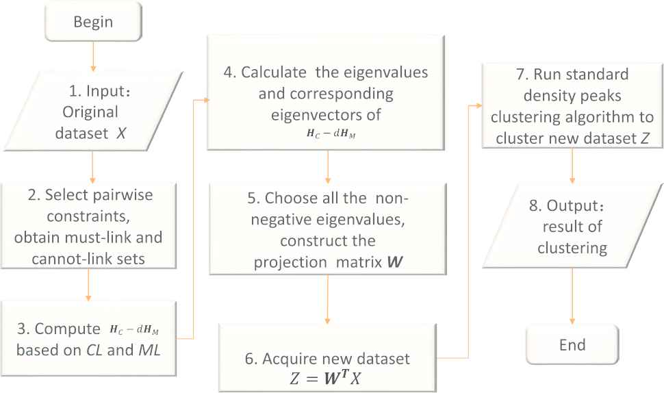
Depiction of the semi-supervised density peaks clustering (SSDPC) algorithm. Steps 1–6 involve the constraint projection of the original dataset
Based on the depiction in Figure 1, the SSDPC algorithm is expressed as follows:
From the process of SSDPC algorithm, we can get complexity of SSDPC model. The time complexity is
SSDPC algorithm:
Input: Dataset
1. Establish the cannot-link set
2. Calculate matrix
3. Compute all the eigenvalues
4. In order to maximize the objective function
5. Use the selected eigenvectors to set up the projection matrix
6. Construct the new dataset
7. Run the standard density peaks clustering (DPC) algorithm on the projected dataset
Output: Clusters
4. EXPERIMENTAL STUDIES
In this section, we describe the experiment settings and performance comparisons for our proposed algorithm SSDPC.
4.1. Datasets Setup
In this part, we investigate the performance of the SSDPC algorithm on a variety of datasets. In the experiments, 17 datasets are acquired from Microsoft Research Asia Multimedia (MSRA-MM) image datasets [39] and three datasets are picked up from the UCI machine learning repository [40]. The details of these 20 datasets are summarized in Table 1.
| Dataset | Characteristic | Classes | Instances | Features |
|---|---|---|---|---|
| Ambulances | Real | 3 | 930 | 892 |
| Aquarium | Real | 3 | 922 | 892 |
| Balloon | Real | 3 | 830 | 892 |
| Bed | Real | 3 | 888 | 892 |
| Birthdaycake | Real | 3 | 932 | 892 |
| Blog | Real | 3 | 943 | 892 |
| Boat | Real | 3 | 857 | 892 |
| Bonsai | Real | 3 | 867 | 892 |
| Bread | Real | 3 | 885 | 892 |
| Bugat | Real | 3 | 882 | 892 |
| Building | Real | 3 | 911 | 892 |
| Bus | Real | 3 | 910 | 892 |
| Butterflytattoo | Real | 3 | 738 | 892 |
| Cactus | Real | 3 | 919 | 892 |
| Credit approval | Mixed | 2 | 690 | 15 |
| Vertebral column | Real | 2 | 310 | 6 |
| Vista | Real | 3 | 799 | 899 |
| Vistawallpaper | Real | 3 | 799 | 899 |
| Voituretuning | Real | 3 | 879 | 899 |
| Congressional voting records | Discrete | 2 | 453 | 16 |
Characteristics, classes, the quantity of instances, and features in each dataset.
The MSRA-MM dataset was assembled from a commercial search engine with more than 1 million images and 20 thousand videos. The purpose of MSRA-MM is to promote research in the field of multimedia information retrieval and related areas. Seventeen image datasets are chosen for the assignment of semi-supervised density peaks clustering (DPC). Each image dataset embraces practically 1,000 instances with nearly 900 features.
UCI Machine Learning Repository currently maintains 507 datasets as a service to the machine learning communities for experimental studies of machine learning methods. New datasets are constantly supported by researchers' donations from all over the world. The most popular UCI datasets are Iris, Cancer, Wine, Breast, Heart Disease, Bank Marketing, Adult, Car Evaluation, Forest Fires, Wisconsin (Diagnostic), Human Activity Recognition Using Smartphones, Wine Quality, Poker Hand, and Abalone. In this empirical analysis, we pick credit approval, vertebral column, and congressional voting records from the UCI datasets. The particulars of each dataset, including classes, the quantity of instances, and features are tabulated in Table 1.
4.2. Experiments
To evaluate how the proposed SSDPC algorithm performs, three other contemporary semi-supervised learning algorithms, constrained k-means clustering with background knowledge (Cop-kmeans) [2], constrained 1-spectral clustering (COSC) [41], and semi-supervised clustering based on affinity propagation (Semi-AP) [42] are also implemented. All experiments are organized on a computer with Intel (R) Core (TM) i5-4460M CPU 3.20 GHz and 4.00 GB RAM, running Matlab R2010b. Each algorithm experiment is repeated 10 times on the 20 datasets.
The crucial modification of Cop-kmeans is to make sure none of the specified constraints are violated when updating cluster assignments. Cop-kmeans allots each point
Parameters for Cop-kmeans, COSC, and Semi-AP are all determined as described in the original studies [2,41,42].
The proposed algorithm SSDPC is implemented in accordance with the depiction in Figure 1. In this case, 10% of pairwise constraints information are applied to construct the
For the evaluation measurement, we apply micro-averaged-precision (
4.3. Results and Discussion
In this part, results of our experiments are provided. Table 2 shows the accuracy results of the different algorithms on 20 datasets. Records are tabulated in terms of averaged mean accuracies and standard deviations over 10 repetitions of the experiments. The mean accuracies of the SSDPC algorithm are higher than the other three semi-supervised learning algorithms (Cop-kmeans, Semi-SC, Semi-AP) on the 20 different datasets, and the highest accuracy value is for the congressional voting records dataset, which reaches 0.8805. The proposed SSDPC algorithm also has the highest average accuracy for all datasets with an average MAP value of 0.5797.
| Datasets | Cop-kmeans | COSC | Semi-AP | SSDPC |
|---|---|---|---|---|
| Ambulances | 0.4512 ± 0.0435 | 0.3967 ± 0.0371 | 0.4261 ± 0.0271 | 0.5970 ± 0.0536 |
| Aquarium | 0.4344 ± 0.0493 | 0.3989 ± 0.0560 | 0.4055 ± 0.0270 | 0.6505 ± 0.0731 |
| Balloon | 0.4536 ± 0.0416 | 0.3796 ± 0.0277 | 0.4589 ± 0.0452 | 0.5530 ± 0.0409 |
| Bed | 0.4468 ± 0.0592 | 0.4314 ± 0.0822 | 0.4337 ± 0.0418 | 0.5680 ± 0.0702 |
| Birthdaycake | 0.5004 ± 0.0264 | 0.3820 ± 0.0354 | 0.4923 ± 0.0257 | 0.5599 ± 0.0514 |
| Blog | 0.4467 ± 0.0590 | 0.4340 ± 0.0680 | 0.4060 ± 0.0351 | 0.5883 ± 0.0891 |
| Boat | 0.4288 ± 0.0585 | 0.4260 ± 0.0571 | 0.4097 ± 0.0347 | 0.5718 ± 0.0819 |
| Bonsai | 0.3978 ± 0.0393 | 0.3973 ± 0.0406 | 0.4321 ± 0.0334 | 0.5608 ± 0.0924 |
| Bread | 0.4660 ± 0.0225 | 0.4546 ± 0.0801 | 0.4460 ± 0.0513 | 0.5786 ± 0.0615 |
| Bugat | 0.4418 ± 0.0600 | 0.4206 ± 0.0568 | 0.4011 ± 0.0388 | 0.5808 ± 0.0814 |
| Building | 0.5568 ± 0.0608 | 0.4617 ± 0.0920 | 0.4651 ± 0.0619 | 0.6422 ± 0.0709 |
| Bus | 0.4700 ± 0.0384 | 0.4163 ± 0.0777 | 0.4293 ± 0.0359 | 0.5522 ± 0.0675 |
| Butterflytattoo | 0.6070 ± 0.0572 | 0.3737 ± 0.0204 | 0.5680 ± 0.0235 | 0.6347 ± 0.0634 |
| Cactus | 0.4868 ± 0.0753 | 0.4132 ± 0.0631 | 0.4771 ± 0.0574 | 0.5929 ± 0.0679 |
| Credit approval | 0.6162 ± 0.0142 | 0.5868 ± 0.0180 | 0.5619 ± 0.0007 | 0.6446 ± 0.0268 |
| Vertebral column | 0.6955 ± 0.0216 | 0.6448 ± 0.0652 | 0.6697 ± 0.0436 | 0.7177 ± 0.0671 |
| Vista | 0.4426 ± 0.0410 | 0.3930 ± 0.0234 | 0.4464 ± 0.0291 | 0.5601 ± 0.0834 |
| Vistawallpaper | 0.4451 ± 0.0326 | 0.4126 ± 0.0814 | 0.4606 ± 0.0207 | 0.5603 ± 0.0652 |
| Voituretuning | 0.4207 ± 0.0288 | 0.4354 ± 0.1005 | 0.4243 ± 0.0365 | 0.5994 ± 0.0643 |
| Congressional voting records | 0.8678 ± 0.0141 | 0.5460 ± 0.0311 | 0.8618 ± 0.0138 | 0.8805 ± 0.0184 |
| Average | 0.5038 | 0.4402 | 0.4839 | 0.5797 |
COSC, constrained 1-spectral clustering; SSDPC, semi-supervised density peaks clustering; AP, affinity propagation.
Performance of different algorithms in terms of accuracy on 20 datasets (mean
To provide a robust comparison among the four algorithms, we carry out a
| Datasets | Cop-kmeans | COSC | Semi-AP | SSDPC | Total |
|---|---|---|---|---|---|
| Ambulances | −0.0166(40) | −0.0711(74) | −0.0416(60) | 0.1292(3) | 177 |
| Aquarium | −0.0380(55) | −0.0734(75) | −0.0668(71) | 0.1782(1) | 202 |
| Balloon | −0.0077(33) | −0.0817(77) | −0.0024(31) | 0.0917(13) | 154 |
| Bed | −0.0231(45) | −0.0386(56) | −0.0363(52) | 0.0980(11) | 164 |
| Birthdaycake | 0.0168(26) | −0.1017(78) | 0.0086(29) | 0.0762(19) | 152 |
| Blog | −0.0221(44) | −0.0347(51) | −0.0627(69) | 0.1196(5) | 169 |
| Boat | −0.0303(47) | −0.0331(49) | −0.0494(64) | 0.1127(7) | 167 |
| Bonsai | −0.0492(62) | −0.0497(65) | −0.0149(37) | 0.1138(6) | 170 |
| Bread | −0.0203(43) | −0.0317(48) | −0.0403(57) | 0.0923(12) | 160 |
| Bugat | −0.0193(42) | −0.0405(58) | −0.0600(68) | 0.1197(4) | 172 |
| Building | 0.0253(24) | −0.0697(73) | −0.0663(70) | 0.1107(8) | 175 |
| Bus | 0.0030(30) | −0.0507(66) | −0.0376(54) | 0.0852(17) | 167 |
| Butterflytattoo | 0.0612(21) | −0.1722(79) | 0.0222(25) | 0.0888(16) | 141 |
| Cactus | −0.0057(32) | −0.0794(76) | −0.0154(38) | 0.1004(9) | 155 |
| Credit approval | 0.0138(27) | −0.0156(39) | −0.0405(59) | 0.0422(22) | 147 |
| Vertebral column | 0.0135(28) | −0.0371(53) | −0.0123(35) | 0.0358(23) | 139 |
| Vista | −0.0180(41) | −0.0675(72) | −0.0141(36) | 0.0996(10) | 159 |
| Vistawallpaper | −0.0246(46) | −0.0570(67) | −0.0091(34) | 0.0907(15) | 162 |
| Voituretuning | −0.0493(63) | −0.0346(50) | −0.0456(61) | 0.1295(2) | 176 |
| Congressional voting records | 0.0788(18) | −0.2430(80) | 0.0728(20) | 0.0914(14) | 132 |
| Total | 767 | 1286 | 970 | 217 | |
| Average rank | 38.35 | 64.3 | 48.5 | 10.85 |
COSC, constrained 1-spectral clustering; SSDPC, semi-supervised density peaks clustering; AP, affinity propagation.
Aligned results of the four algorithms. The rank value in parentheses are employed in the calculation of the Friedman Aligned Rank test. The lowest rank value is the best one.
In the above two formulas,
With four algorithms and 20 datasets,
5. CONCLUSION AND PROSPECTS
In this paper, we present a new SSDPC using pairwise constraints, as it is simpler to obtain pairwise constraint information than to acquire class tags (or labels). We consider applying pairwise constraint knowledge to project the original data onto a well-preserved lower dimensional space, which forces the distance between instances in ML pairs) to be decreased and the distance between instances in
As various data is achievable in daily life, for instance, signal lights data, railway track circuit data, diagnostic data, and so on. Applying the proposed SSDPC algorithm in analyzing different kinds of data is practicable. As we know, clustering by using density peaks is an efficient method when it was proposed in 2014 [23]. In this work, we extend DPC algorithm to a semi-supervised learning algorithm, the results show the semi-DPC algorithm is feasible. However, the algorithm is still robust with the value of cutoff distance
CONFLICTS OF INTEREST
The authors declare they have no conflicts of interest.
AUTHORS' CONTRIBUTIONS
All authors contributed to this study. All authors read and approved the final manuscript.
ACKNOWLEDGMENTS
This research is supported by the National Natural Science Foundation of China for Youth (Grant No. 61703349), Science and Technology research and development project of China Railway Corporation (Grant No. N2018G062, K2018G011).
REFERENCES
Cite this article
TY  - JOUR
AU  - Shan Yan
AU  - Hongjun Wang
AU  - Tianrui Li
AU  - Jielei Chu
AU  - Jin Guo
PY  - 2020
DA  - 2020/11/09
TI  - Semi-Supervised Density Peaks Clustering Based on Constraint Projection
JO  - International Journal of Computational Intelligence Systems
SP  - 140
EP  - 147
VL  - 14
IS  - 1
SN  - 1875-6883
UR  - https://doi.org/10.2991/ijcis.d.201102.002
DO  - 10.2991/ijcis.d.201102.002
ID  - Yan2020
ER  -