
Flexible Bootstrap for Fuzzy Data Based on the Canonical Representation
 , Olgierd Hryniewicz2, Maciej Romaniuk2, 3
- DOI
- 10.2991/ijcis.d.201012.003How to use a DOI?
- Keywords
- Ambiguity; Bootstrap; Canonical representation; Fuzziness; Fuzzy data; Fuzzy numbers; Random fuzzy numbers; Resampling
- Abstract
Several new resampling methods for generating bootstrap samples of fuzzy numbers are proposed. To avoid undesired repetitions in the secondary samples we do not draw randomly directly observations from the primary samples but construct them allowing for some modifications in their membership functions, however only such which do not disturb the canonical representation of the initial fuzzy numbers. We consider both two-parameter and three-parameter canonical representations, as well as the triangular and trapezoidal outputs in the secondary samples. Numerical experiments concerning some statistical tests based on fuzzy samples show that the suggested methods may appear helpful in statistical reasoning with imprecise data.
- Copyright
- © 2020 The Authors. Published by Atlantis Press B.V.
- Open Access
- This is an open access article distributed under the CC BY-NC 4.0 license (http://creativecommons.org/licenses/by-nc/4.0/).
1. INTRODUCTION
The bootstrap, introduced by Efron [1], is a widespread statistical technique for assessing uncertainty and solving various complex problems. For instance, it appears extremely useful for estimating standard errors, for computing confidence intervals or testing hypotheses in all those cases where no theoretical results are available and using normal approximation or any other parametric approach remains questionable.
Such a situation is typical in statistical inference based on imprecise data modelled with fuzzy numbers. Indeed, in most cases when the analyzed phenomena is described by fuzzy random variables (random fuzzy numbers) the underlying distribution remains unknown. There, the bootstrap is as not only helpful but sometimes appears as the onliest tool to conduct any statistical reasoning. In particular, the bootstrap was successfully applied in statistical tests for fuzzy data by Colubi et al. [2], Gil et al. [3], González-Rodríguez et al. [4,5], Grzegorzewski and Ramos-Guajardo [6], Montenegro et al. [7] and Ramos-Guajardo and Lubiano [8]. Some examples on the bootstrap application for solving the real-life problems include, e.g., fuzzy questionnaires rating (Ref. [9]), also in cheese manufacturing (Ref. [10]) or fuzzy control charts (Ref. [11]).
The main idea of the classical bootstrap consists in drawing random samples with replacement from the initial sample of the experiment outcomes and then construct the empirical distribution through averaging the bootstrap samples. Such procedure, although simple yet efficient, has an important disadvantage: in the generated secondary samples we obtain only the values belonging to the initial (primary) sample and hence, nearly every bootstrap sample contains repeated values. If the primary sample size is small, all bootstrap samples consist of only few distinct values. Such a case seems to be strange especially if the unknown original distribution is continuous. To overcome this inconvenience some modifications and improvements of the classical bootstrap were proposed, like the balanced bootstrap by Davison et al. [12] or Graham et al. [13], as well as various kinds of the so-called smoothed bootstrap discussed by Silverman and Young [14], Hall et al. [15] or De Angelis and Young [16].
Excessive repetitions in bootstrap samples is also a problem in fuzzy modelling. To increase the diversity of simulated results some new approaches were proposed. Romaniuk and Hryniewicz [17,18] introduced two resampling methods in which new triangular fuzzy numbers were generated from the primary sample by adding some incremental spreads for
In this paper, we propose another modification of the bootstrap approach which prevents from undesired repetitions in secondary fuzzy sample generation. Our key idea is to generate such triangular or trapezoidal fuzzy numbers which have the same canonical representations as fuzzy observations in the primary sample. As it is known, the canonical representation of a fuzzy number, proposed by Delgado et al. [20], summarizes information on basic characteristics of a fuzzy number. Obviously, two fuzzy numbers with identical canonical representation may have membership functions which differ a little bit. Thus by generating fuzzy numbers with the fixed canonical representation, we may obtain secondary samples with desired characteristics but without replicating observations from the initial sample. This is the reason why the aforementioned bootstrap idea was called flexible.
Flexible bootstrap was suggested for the first time in Ref. [21], where the algorithm for generating fuzzy numbers with fixed two-parameter canonical representation, i.e., the value and ambiguity, was considered. In this paper, we examine extensively this kind of the flexible bootstrap for triangular and trapezoidal fuzzy numbers. Moreover, we introduce another flexible bootstrap algorithm dedicated to trapezoidal fuzzy numbers which preserves three-parameter canonical representation comprising the value, ambiguity and the fuzziness of a fuzzy number.
This paper is organized as follows: In Section 2 we recall basic definitions and concepts related to fuzzy numbers and their representation. Section 3 contains a short introduction to random fuzzy numbers. In Section 4 we develop the bootstrap procedures generating triangular and trapezoidal fuzzy numbers which preserve the value and the ambiguity of the initial sample. Then, in Section 5, we propose an algorithm to generate secondary samples of trapezoidal fuzzy numbers that preserve the value, the ambiguity and the fuzziness of observations belonging to the initial sample. In all cases, we provide the resampling algorithms in a form ready for the practical use. In Section 6 we present the results of the real-life case study in which we compare the proposed flexible bootstrap with the classical bootstrap algorithm. Section 7 contains a broad simulation study performed to evaluate some properties of the suggested methods. In particular, we compare the empirical size and the power of two one-sample tests and the two-sample test equipped with the standard bootstrap procedure and our flexible bootstrap algorithms. We also discuss the standard error of estimators based on the proposed bootstrap algorithms.
2. FUZZY NUMBERS AND THEIR CHARACTERISTICS
As the most often type of data used in classical statistical inference are real-valued observations, i.e., real numbers or vectors of reals, the same happens in fuzzy environment where the central role is played by fuzzy numbers. Indeed, although various types of fuzzy sets are considered for modelling imprecision, just fuzzy numbers are actually used most often.
A fuzzy number
An
Membership functions of fuzzy numbers may assume different shapes. However, the most often used fuzzy numbers are the trapezoidal fuzzy numbers with membership functions of the form
Instead of declaring two points
Here
One may ask why to restrict our attention to triangular or trapezoidal fuzzy numbers only. The reason is straightforward: it is due to their simplicity. Trapezoidal or triangular fuzzy numbers are easy to handle and have a natural interpretation. Moreover, even if the original data set consists of fuzzy numbers which are neither triangular nor trapezoidal, one may easily approximate them by such fuzzy numbers. In particular, an approximation algorithm which preserves the value and the ambiguity of the original fuzzy number is given in Ref. [22], while the broad collection of approximation methods satisfying various requirements can be found in Ref. [23].
To simplify the representation of fuzzy numbers Delgado et al. [20] suggested two parameters — the value and the ambiguity — which characterize two basic features of a fuzzy number and hence were called together as the canonical representation of a fuzzy number.
The first characteristic called the value and defined as follows:
Some straightforward calculations show that the value and the ambiguity of a trapezoidal fuzzy number
Obviously, if
As advocated by Delgado et al., the value and the ambiguity represent basic features of a fuzzy number and therefore two fuzzy numbers with the same ambiguity and the value might be considered as similar (sometimes they are even treated as “almost equal,” see Ref. [20]).
However, since the two-parameter canonical representation of a fuzzy number does not contain the whole information of that fuzzy number we may try to enrich this representation by adding some supplemental parameters. Besides the value and the ambiguity Delgado et al. [20] suggested to consider another characteristic of a fuzzy number, called its fuzziness. The fuzziness tries to quantify the difference between a fuzzy number and its complement and is defined as follows:
One can find that the fuzziness of a trapezoidal fuzzy number
Hence, if
On the other hand, for the trapezoidal fuzzy number
One can define various metrics in
For more details on fuzzy numbers, their types and characteristics we refer the reader to Ref. [23].
3. RANDOM FUZZY NUMBERS
To analyze fuzzy data and to conduct a statistical inference we need a formal model for the random mechanism generating fuzzy number-valued data. Such model should integrate randomness, associated with data generation mechanism and fuzziness, connected with the intrinsic nature of the data, i.e., their imprecision.
To cope with this problem Puri and Ralescu [26] introduced the notion of a fuzzy random variable, also called a random fuzzy number.
Definition 1.
Given a probability space
Alternatively,
Puri and Ralescu [26] defined also the Aumann-type mean of a fuzzy random variable
So defined
To characterize dispersion of a fuzzy random variable
Although random fuzzy numbers preserve some properties known from the real-valued inference, one should be aware of the problems typical of statistical reasoning with fuzzy data. In particular, due to the nonlinearities of the space of fuzzy numbers it is advisable to avoid subtraction of fuzzy numbers wherever it is possible (the same hold for the division). Some difficulties in fuzzy data analysis may be caused by the lack of universally accepted total ranking between fuzzy numbers. Another source of possible crucial problems that appear in conjunction of randomness and fuzziness is the absence of suitable models for the distribution of fuzzy random variables. Moreover, there are not yet Central Limit Theorems for fuzzy random variables which can be applied directly in statistical inference.
The aforementioned arguments could strongly discourage statistical inference with fuzzy data if not the two brilliant ideas that indicate the way-out in this situation. Firstly, in the late 1970s Efron [1] developed the bootstrap method to approximate the distribution of inferential statistics when the population distribution is unknown. Next, in the very early 1990s Giné and Zinn [27] developed a bootstrapped approximation to the CLT for generalized random elements, which opens the door for the bootstrap application in statistical inference with fuzzy data.
4. VALUE-AMBIGUITY (VA) BOOTSTRAP ALGORITHM
To avoid undesired repetitions which often appear in bootstrap Romaniuk and Hryniewicz [17–19] proposed a resampling method which enrich secondary samples with fuzzy observations imitating those from the primary sample but containing some incremental spreads on their
4.1. VA Algorithm for Triangular Observations
Let
Let us compute the value and the ambiguity of each observation in this primary sample following Eqs. (2) and (3). This way we obtain a set of pairs
The main idea of the proposed bootstrap technique is to create a secondary sample by generating randomly fuzzy observations from the set (12). Obviously, although the value and the ambiguity characterize nicely a fuzzy number, they do not identify it completely. Thus by imposing some restrictions on the generated fuzzy numbers we have still some room for the choice of their membership function. Let us retrace in detail how it works.
In this section we assume that the desired secondary sample
Let
Moreover, by the definition,
We can gather all these considerations in the following bootstrap algorithm.
Thus, following Algorithm 1 we receive the secondary bootstrap sample
Algorithm 1
Given a fuzzy sample
Let
Draw randomly (with equal probabilities) a pair
Generate a random value
Compute
Compute
Let
If
4.2. VA Algorithm for Trapezoidal Observations
As before, let
Since
Summing up the aforementioned considerations as well as restrictions specified in (15), (16) and (17), we obtain the following bootstrap algorithm for generating a secondary sample of trapezoidal fuzzy numbers.
Therefore, Algorithm 2 provides a bootstrap secondary sample
Algorithm 2
Given a fuzzy sample
Let
Draw randomly (with equal probabilities) a pair
Generate a random value
Generate a random value
Compute
Compute
Let
If
5. VALUE-AMBIGUITY-FUZZINESS (VAF) BOOTSTRAP ALGORITHM
Both algorithms proposed in Sections 4.1 and 4.2 show how to generate secondary bootstrap samples which preserve the value and ambiguity of observations from the initial sample. While keeping track of those algorithms one may notice that by fixing two-parameter canonical representation of a fuzzy number we have something like “one degree of freedom” in generating a triangular fuzzy number and “two degrees of freedom” in trapezoidal fuzzy number generation. Indeed, besides drawing randomly a pair
One way to reduce the number of undesired “degrees of freedom” in generating bootstrap samples which consist of trapezoidal fuzzy numbers is to consider a more extended canonical representation of a fuzzy number, i.e., to fix another characteristic besides its value and ambiguity. A possible candidate is the fuzziness described in Section 2.
Indeed, by computing not only the value and the ambiguity of each observation from the primary sample
Next, assuming that the desired secondary sample
Summing up the aforementioned considerations as well as the restrictions specified in (15), (16) and (17), we obtain the following bootstrap algorithm for generating a secondary sample of trapezoidal fuzzy numbers.
Therefore, Algorithm 3 provides the bootstrap secondary sample
Example 1.
Let us assume that
Then, according to step 5 of Algorithm 3, we generate randomly
Algorithm 3
Given a fuzzy sample
Let
Draw randomly (with equal probabilities) a triple
Compute
Generate a random value
Compute
Compute
Let
If
6. CASE STUDY
Resampling techniques are commonly used to solve practical problems [9–11], therefore we compare the introduced algorithms also in the case of a real-life application. We utilize some data [10] related to the quality of the Gamonedo cheese, which is a kind of blue cheese produced in Asturias, Spain. Some of its testers expressed their subjective opinions using trapezoidal fuzzy numbers and we compare the overall impressions of three experts about this cheese [8,10].
To compare the means of two independent samples, i.e., to verify the hypothesis
We compare pairwise the mean opinions of the three previously mentioned experts (Expert A, B and C) to check if they have “similar overall opinions.” In the case of two pairs (Expert A vs. Expert B and Expert B vs. Expert C), all the resampling approaches for the C2-test give the same estimated p value about 0.0000 (even for
| 100 | 200 | 1000 | |
|---|---|---|---|
| Boot. | 0.8 | 0.835 | 0.84 |
| VA | 0.96 | 0.955 | 0.941 |
| VAF | 0.87 | 0.86 | 0.848 |
Empirical p values for the C2-test concerning the quality of the Gamonedo cheese (Expert A vs. C).
7. SIMULATION STUDY
7.1. One-Sample Tests
Hypotheses testing with fuzzy data attract attention of many researches (see, e.g., Refs. [3,5–8,31]) and most of the cited papers utilize bootstrap methods to determine a null distribution under study. This is the reason that we also examine our new bootstrap methods suggested in this contribution with three tests for the expected value. The first one is a bootstrapped version of the Körner test [31], the second one is developed by Montenegro et al. [5,7] and the third one (related also to the second test) is discussed by Colubi [30] and Lubiano et al. [9]. Further on, they will be denoted as the K-test, the M-test and the C-test, respectively. All these tests were designed to verify the following problem
We consider a few types of fuzzy numbers (summarized in Table 2) to create primary fuzzy random sample
| Type | c | s | l | r |
|---|---|---|---|---|
| N(0,1) | – | |||
| N(0,1) | – | Exp(2) | Exp(4) | |
| N(0,1) | – | U(0,0.4) | U(0,0.4) | |
| N(0,1) | U(0,0.1) | U(0,0.1) | U(0,0.3) | |
| U(0,0.2) | Exp(4) | Exp(2) |
Description of types of the simulated fuzzy numbers.
Similarly, the centers for
For each type of fuzzy numbers, initial random samples of size
As the essential benchmark, we use the empirical size of the test
Results given in Tables 3–8 show that both the classical approach (denoted by “Boot.”) and the suggested VA resampling procedure are very close to each other. It seems that the empirical sizes of the test
| 5 | 10 | 30 | 100 | |
|---|---|---|---|---|
| 100 | ||||
| Boot. | 0.16024 | 0.10113 | 0.07006 | 0.06331 |
| VA | 0.15954 | 0.10476 | 0.07616 | 0.06814 |
| 200 | ||||
| Boot. | 0.15438 | 0.09686 | 0.0658 | 0.05795 |
| VA | 0.15236 | 0.09833 | 0.0711 | 0.06207 |
| 1000 | ||||
| Boot. | 0.14834 | 0.0911 | 0.06297 | 0.05449 |
| VA | 0.14523 | 0.09421 | 0.06519 | 0.0585 |
Empirical K-test size
| 5 | 10 | 30 | 100 | |
|---|---|---|---|---|
| 100 | ||||
| Boot. | 0.17437 | 0.1078 | 0.07297 | 0.0633 |
| VA | 0.168 | 0.10542 | 0.07108 | 0.05378 |
| 200 | ||||
| Boot. | 0.16529 | 0.10371 | 0.06852 | 0.05739 |
| VA | 0.16395 | 0.10009 | 0.06591 | 0.04933 |
| 1000 | ||||
| Boot. | 0.16155 | 0.09762 | 0.06543 | 0.05515 |
| VA | 0.15952 | 0.09628 | 0.06162 | 0.04674 |
Empirical K-test size
| 5 | 10 | 30 | 100 | |
|---|---|---|---|---|
| 100 | ||||
| Boot. | 0.17553 | 0.10833 | 0.07303 | 0.06285 |
| VA | 0.17183 | 0.10803 | 0.07445 | 0.06319 |
| 200 | ||||
| Boot. | 0.16669 | 0.10309 | 0.06878 | 0.05775 |
| VA | 0.16806 | 0.1021 | 0.06895 | 0.05746 |
| 1000 | ||||
| Boot. | 0.16255 | 0.0977 | 0.06584 | 0.0556 |
| VA | 0.16352 | 0.09843 | 0.06432 | 0.05432 |
Empirical K-test size
| 5 | 10 | 30 | 100 | |
|---|---|---|---|---|
| 100 | ||||
| Boot. | 0.03375 | 0.04906 | 0.0562 | 0.05892 |
| VA | 0.0339 | 0.04347 | 0.0489 | 0.05107 |
| 200 | ||||
| Boot. | 0.02988 | 0.04449 | 0.05196 | 0.05473 |
| VA | 0.02915 | 0.03915 | 0.04493 | 0.04597 |
| 1000 | ||||
| Boot. | 0.02748 | 0.04047 | 0.04916 | 0.05064 |
| VA | 0.02603 | 0.03567 | 0.04078 | 0.0423 |
Empirical M-test size
| 5 | 10 | 30 | 100 | |
|---|---|---|---|---|
| 100 | ||||
| Boot. | 0.03634 | 0.05033 | 0.05777 | 0.05862 |
| VA | 0.03724 | 0.04912 | 0.05488 | 0.05569 |
| 200 | ||||
| Boot. | 0.03095 | 0.04593 | 0.05286 | 0.05344 |
| VA | 0.03248 | 0.04367 | 0.04989 | 0.04911 |
| 1000 | ||||
| Boot. | 0.02871 | 0.04107 | 0.05009 | 0.05087 |
| VA | 0.02997 | 0.04058 | 0.04564 | 0.0469 |
Empirical M-test size
| 5 | 10 | 30 | 100 | |
|---|---|---|---|---|
| 100 | ||||
| Boot. | 0.03246 | 0.04915 | 0.05742 | 0.05851 |
| VA | 0.03352 | 0.05026 | 0.0588 | 0.05903 |
| 200 | ||||
| Boot. | 0.02663 | 0.04431 | 0.05325 | 0.05327 |
| VA | 0.02832 | 0.04433 | 0.05351 | 0.05314 |
| 1000 | ||||
| Boot. | 0.02381 | 0.04006 | 0.04954 | 0.05113 |
| VA | 0.02612 | 0.04026 | 0.04874 | 0.05046 |
Empirical M-test size
Going into details, when discussing the K-test (Tables 3–5), it seems that the VA method dominates the classical bootstrap for
In the case of the M-test (see Tables 6–8), the general comparison of the classical bootstrap and the VA method shows that there is also no apparent winner: for small sample sizes sometimes the VA method is better, otherwise the classical approach dominates. When we compare the situation under the different number of bootstrap repetitions no obvious conclusion imposes.
In the case of trapezoidal fuzzy numbers, the C-test is applied to compare the empirical sizes for this test using the classical bootstrap, the VA method and the VAF method with the same values of
In general, as we can see from Tables 9 and 10, there are some significant differences, especially for small
| 5 | 10 | 30 | 100 | |
|---|---|---|---|---|
| 100 | ||||
| Boot. | 0.03072 | 0.04896 | 0.05818 | 0.05847 |
| VA | 0.03137 | 0.04862 | 0.0574 | 0.05772 |
| VAF | 0.03217 | 0.04862 | 0.05778 | 0.05716 |
| 200 | ||||
| Boot. | 0.02581 | 0.04435 | 0.05217 | 0.05519 |
| VA | 0.02613 | 0.04367 | 0.05331 | 0.05394 |
| VAF | 0.02512 | 0.04385 | 0.05125 | 0.05383 |
| 1000 | ||||
| Boot. | 0.0232 | 0.03982 | 0.04966 | 0.05156 |
| VA | 0.02414 | 0.03989 | 0.04856 | 0.04929 |
| VAF | 0.02379 | 0.04037 | 0.04978 | 0.0494 |
Empirical C-test size
| 5 | 10 | 30 | 100 | |
|---|---|---|---|---|
| 100 | ||||
| Boot. | 0.05272 | 0.0676 | 0.06291 | 0.05947 |
| VA | 0.05397 | 0.06602 | 0.05956 | 0.0554 |
| VAF | 0.05353 | 0.06561 | 0.06036 | 0.05624 |
| 200 | ||||
| Boot. | 0.04773 | 0.06349 | 0.05781 | 0.05507 |
| VA | 0.04755 | 0.06168 | 0.05507 | 0.05049 |
| VAF | 0.04802 | 0.06073 | 0.05518 | 0.05028 |
| 1000 | ||||
| Boot. | 0.04456 | 0.05935 | 0.05424 | 0.05162 |
| VA | 0.04511 | 0.05763 | 0.05193 | 0.04718 |
| VAF | 0.04545 | 0.05777 | 0.05118 | 0.0483 |
Empirical C-test size
Next step of the numerical experiment was the power study of the considered tests equipped with the classical bootstrap, the VA method or the VAF method. Because the null and the alternative hypotheses (22) in these tests concern the strict equality or inequality for a fuzzy number, the respective procedure has to be applied. To examine the power of the tests, we estimated the number of rejections under increasing shift
| 5 | 10 | 30 | 100 | |
|---|---|---|---|---|
| 0.25, 100 | ||||
| Boot. | 0.22496 | 0.199 | 0.3177 | 0.72024 |
| VA | 0.22174 | 0.19778 | 0.31772 | 0.72126 |
| 0.25, 200 | ||||
| Boot. | 0.21777 | 0.19247 | 0.31134 | 0.71411 |
| VA | 0.21791 | 0.19106 | 0.30949 | 0.71335 |
| 0.25, 1000 | ||||
| Boot. | 0.21218 | 0.18781 | 0.30239 | 0.71188 |
| VA | 0.21284 | 0.18705 | 0.30398 | 0.71282 |
| 0.5, 100 | ||||
| Boot. | 0.36195 | 0.43961 | 0.79944 | 0.9987 |
| VA | 0.35853 | 0.43703 | 0.79904 | 0.99864 |
| 0.5, 200 | ||||
| Boot. | 0.35157 | 0.42882 | 0.79486 | 0.99867 |
| VA | 0.35244 | 0.42901 | 0.79472 | 0.99869 |
| 0.5, 1000 | ||||
| Boot. | 0.34748 | 0.42479 | 0.79131 | 0.99885 |
| VA | 0.34767 | 0.42217 | 0.79273 | 0.99893 |
| 0.75, 100 | ||||
| Boot. | 0.54304 | 0.71307 | 0.98386 | 1 |
| VA | 0.54079 | 0.7111 | 0.98425 | 1 |
| 0.75, 200 | ||||
| Boot. | 0.53448 | 0.70511 | 0.98386 | 1 |
| VA | 0.53467 | 0.70805 | 0.9835 | 1 |
| 0.75, 1000 | ||||
| Boot. | 0.52919 | 0.70456 | 0.98447 | 1 |
| VA | 0.52863 | 0.7022 | 0.98363 | 1 |
K-test power analysis for
| 5 | 10 | 30 | 100 | |
|---|---|---|---|---|
| 0.25, 100 | ||||
| Boot. | 0.04708 | 0.1045 | 0.27674 | 0.70835 |
| VA | 0.04763 | 0.10472 | 0.27601 | 0.70968 |
| 0.25, 200 | ||||
| Boot. | 0.03834 | 0.09749 | 0.26958 | 0.70123 |
| VA | 0.04177 | 0.09739 | 0.26873 | 0.70248 |
| 0.25, 1000 | ||||
| Boot. | 0.03571 | 0.09049 | 0.26048 | 0.69996 |
| VA | 0.03792 | 0.0899 | 0.26096 | 0.7012 |
| 0.5, 100 | ||||
| Boot. | 0.08898 | 0.2769 | 0.76116 | 0.99863 |
| VA | 0.08967 | 0.27502 | 0.76064 | 0.9985 |
| 0.5, 200 | ||||
| Boot. | 0.07711 | 0.26214 | 0.75629 | 0.99851 |
| VA | 0.08138 | 0.26332 | 0.75503 | 0.99855 |
| 0.5, 1000 | ||||
| Boot. | 0.07073 | 0.25315 | 0.75066 | 0.99871 |
| VA | 0.07326 | 0.25213 | 0.75301 | 0.9988 |
| 0.75, 100 | ||||
| Boot. | 0.15996 | 0.52679 | 0.97706 | 1 |
| VA | 0.16177 | 0.52473 | 0.97759 | 1 |
| 0.75, 200 | ||||
| Boot. | 0.14084 | 0.51102 | 0.97743 | 1 |
| VA | 0.14723 | 0.51362 | 0.97705 | 1 |
| 0.75, 1000 | ||||
| Boot. | 0.13156 | 0.50551 | 0.97771 | 1 |
| VA | 0.13547 | 0.50407 | 0.97696 | 1 |
M-test power analysis for
| 5 | 10 | 30 | 100 | |
|---|---|---|---|---|
| 0.25, 100 | ||||
| Boot. | 0.04398 | 0.10497 | 0.28146 | 0.71087 |
| VA | 0.04477 | 0.1037 | 0.2732 | 0.7032 |
| VAF | 0.04481 | 0.10392 | 0.2759 | 0.70426 |
| 0.25, 200 | ||||
| Boot. | 0.03699 | 0.09689 | 0.26573 | 0.69984 |
| VA | 0.03781 | 0.09746 | 0.26485 | 0.69834 |
| VAF | 0.03788 | 0.09595 | 0.26643 | 0.69762 |
| 0.25, 1000 | ||||
| Boot. | 0.03418 | 0.09134 | 0.26152 | 0.69554 |
| VA | 0.03542 | 0.09125 | 0.25929 | 0.69551 |
| VAF | 0.03504 | 0.09157 | 0.25921 | 0.69341 |
| 0.5, 100 | ||||
| Boot. | 0.08472 | 0.27716 | 0.76122 | 0.99878 |
| VA | 0.08738 | 0.27453 | 0.75812 | 0.9985 |
| VAF | 0.08635 | 0.27485 | 0.75776 | 0.99858 |
| 0.5, 200 | ||||
| Boot. | 0.07281 | 0.26274 | 0.75268 | 0.99856 |
| VA | 0.07545 | 0.26151 | 0.75434 | 0.99845 |
| VAF | 0.07443 | 0.26224 | 0.75257 | 0.99858 |
| 0.5, 1000 | ||||
| Boot. | 0.06929 | 0.25442 | 0.75005 | 0.99861 |
| VA | 0.06979 | 0.25425 | 0.75031 | 0.99864 |
| VAF | 0.0695 | 0.25362 | 0.75084 | 0.99852 |
| 0.75, 100 | ||||
| Boot. | 0.15426 | 0.52872 | 0.97674 | 1 |
| VA | 0.15825 | 0.52797 | 0.97722 | 1 |
| VAF | 0.15539 | 0.52695 | 0.97671 | 1 |
| 0.75, 200 | ||||
| Boot. | 0.13543 | 0.51624 | 0.97627 | 1 |
| VA | 0.13981 | 0.51466 | 0.97642 | 1 |
| VAF | 0.13768 | 0.51286 | 0.97652 | 1 |
| 0.75, 1000 | ||||
| Boot. | 0.12831 | 0.50498 | 0.97689 | 1 |
| VA | 0.13004 | 0.50411 | 0.9761 | 1 |
| VAF | 0.12874 | 0.5044 | 0.97615 | 1 |
C-test power analysis for
| 5 | 10 | 30 | 100 | |
|---|---|---|---|---|
| 0.25, 100 | ||||
| Boot. | 0.04212 | 0.0515 | 0.05583 | 0.12237 |
| VA | 0.04307 | 0.04998 | 0.05405 | 0.11691 |
| VAF | 0.04296 | 0.05006 | 0.05595 | 0.11479 |
| 0.25, 200 | ||||
| Boot. | 0.03758 | 0.04651 | 0.05078 | 0.11361 |
| VA | 0.0373 | 0.04573 | 0.04919 | 0.10843 |
| VAF | 0.03785 | 0.04569 | 0.04761 | 0.1092 |
| 0.25, 1000 | ||||
| Boot. | 0.03521 | 0.04368 | 0.04592 | 0.10715 |
| VA | 0.03519 | 0.04228 | 0.04447 | 0.09967 |
| VAF | 0.03526 | 0.04226 | 0.04523 | 0.10037 |
| 0.5, 100 | ||||
| Boot. | 0.03465 | 0.04794 | 0.10707 | 0.40581 |
| VA | 0.0361 | 0.04705 | 0.10309 | 0.392 |
| VAF | 0.03574 | 0.04742 | 0.10425 | 0.38931 |
| 0.5, 200 | ||||
| Boot. | 0.03052 | 0.04251 | 0.09776 | 0.39256 |
| VA | 0.03056 | 0.04204 | 0.09466 | 0.38094 |
| VAF | 0.03006 | 0.04246 | 0.09413 | 0.38102 |
| 0.5, 1000 | ||||
| Boot. | 0.0291 | 0.03849 | 0.09125 | 0.38409 |
| VA | 0.02877 | 0.03804 | 0.08657 | 0.36825 |
| VAF | 0.02841 | 0.03853 | 0.08848 | 0.36717 |
| 0.75, 100 | ||||
| Boot. | 0.03143 | 0.05988 | 0.22716 | 0.77303 |
| VA | 0.03216 | 0.05876 | 0.22043 | 0.75998 |
| VAF | 0.03192 | 0.05932 | 0.21974 | 0.75842 |
| 0.75, 200 | ||||
| Boot. | 0.02642 | 0.05292 | 0.21511 | 0.76798 |
| VA | 0.02719 | 0.05186 | 0.20683 | 0.75334 |
| VAF | 0.02675 | 0.05283 | 0.20829 | 0.75342 |
| 0.75, 1000 | ||||
| Boot. | 0.02489 | 0.04895 | 0.20417 | 0.76269 |
| VA | 0.02511 | 0.04722 | 0.19661 | 0.74743 |
| VAF | 0.02478 | 0.04744 | 0.19837 | 0.74969 |
C-test power analysis for
For
The differences between the bootstrap procedures are hardly discernible especially for the K-test, where it is difficult to designate the real winner. It can be seen also in Figure 1, where the percentages of rejections are shown for some range of smaller values of the shift (i.e.,
Power curves of the K-test for
Power curves of the M-test for
The situation is similar for the considered trapezoidal fuzzy numbers and the C-test (see Tables 13 and 14). The new resampling algorithms are favored for the smallest sample size (i.e.,
Power curves of the C-test for
Power curves of the C-test for
7.2. Two-Sample Tests
In the same manner as in Section 7.1, we conduct a power study for the C2-test. Because of the form of the hypotheses (21), the special approach has to be also applied. The number of rejections is estimated under increasing shift
To shorten the paper, only the results for
Power curves of the C2-test for
Power curves of the C2-test for
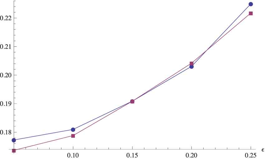
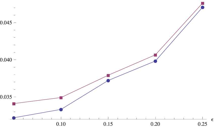
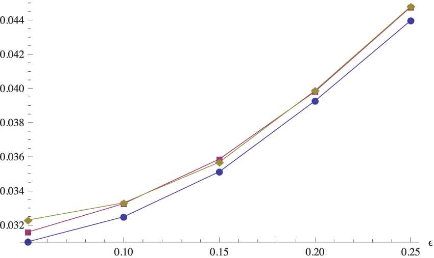
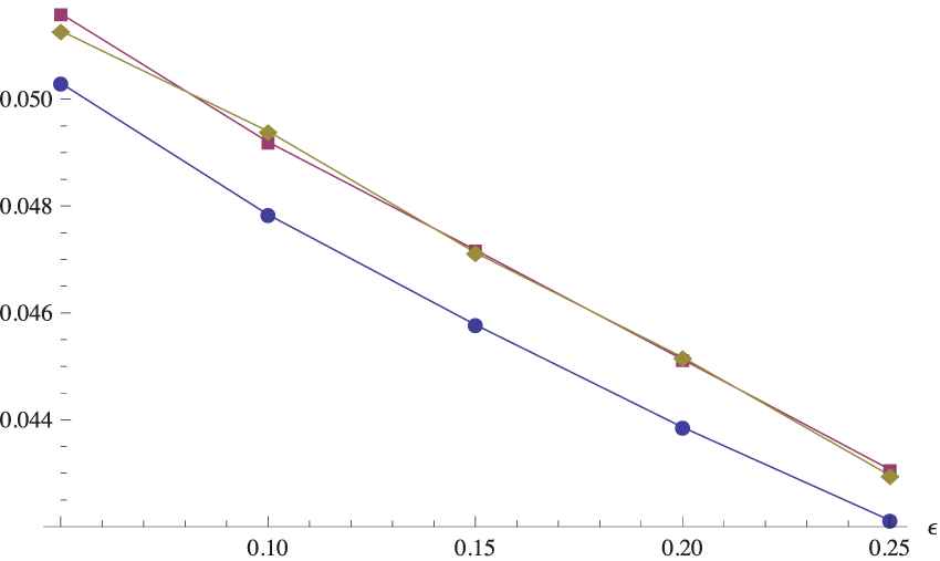
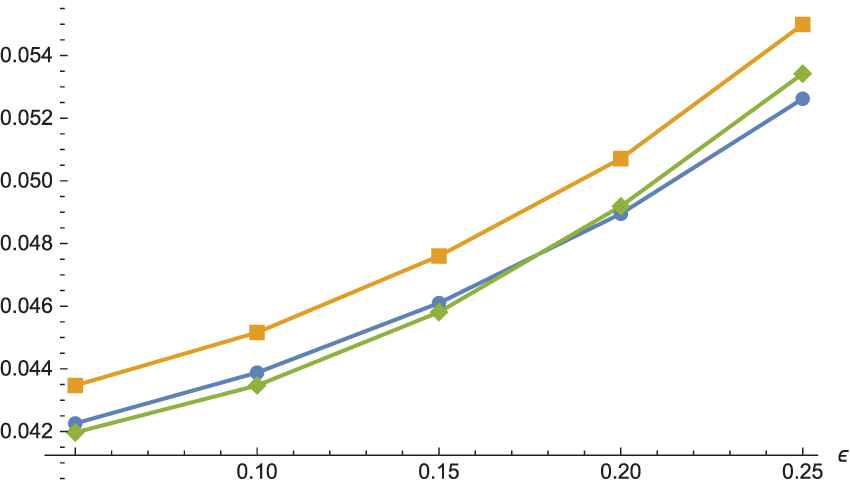
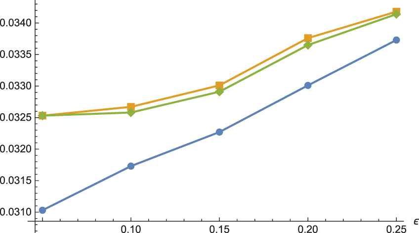
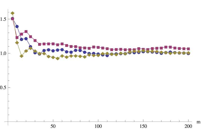
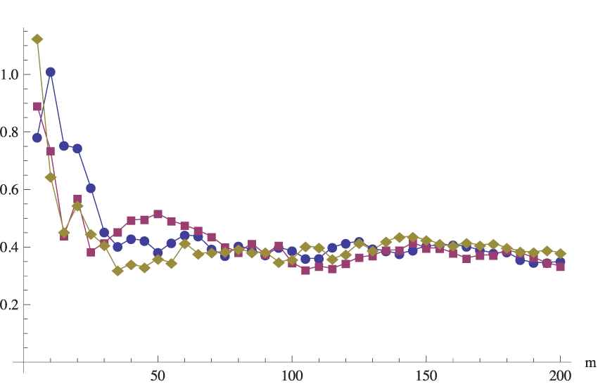
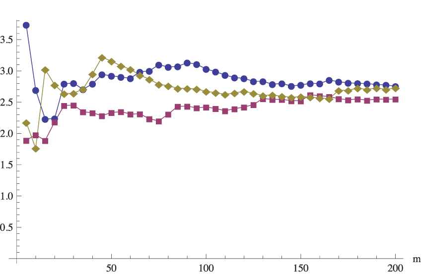
7.3. Standard Error of the Estimators
To evaluate the proposed method for generating bootstrap samples we also analyze the standard error of the estimators of the mean obtained from the secondary samples based on the classical approach, the VA and the VAF method. We consider the following two estimators of the variance (12), namely
To shorten the paper, we provide the results only for the two cases of a moderate size (
SE1(m) for the moderate primary sample
SE2(m) for the moderate primary sample
SE1(m) for the moderate primary sample
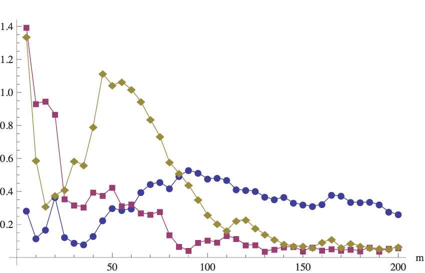
SE2(m) for the moderate primary
It seems that the obtained variabilities tend to be similar for all sampling methods, but in the case of
8. CONCLUSIONS
Various methods to avoid undesired repetitions in the bootstrap samples have been proposed in the literature. In this paper, we suggest another approach, called the flexible bootstrap, which can help to enrich bootstrap samples of fuzzy numbers. Our main idea is to substitute the process of drawing randomly observations from the primary samples and inserting them directly into the secondary sample by the more sophisticated approach, where the members of the secondary sample may somehow differ from those that appear in the primary one. We simply allow for some modifications in their membership functions, however only such which do not disturb the canonical representation of the initial fuzzy numbers. We consider both two-parameter (the value and the ambiguity) and three-parameter (the value, the ambiguity and the fuzziness) canonical representations. Then we present three algorithms for generating bootstrap samples of triangular or trapezoidal fuzzy numbers which preserve the canonical representations of observations from the primary sample.
The aforementioned algorithms for generating bootstrap samples are presented in the form ready for direct use by the practitioners. Moreover, the proposed methods were examined through the broad simulation study focused on two statistical tests and compared with the classical bootstrap. The promising results indicate that the suggested methodology can be useful in statistical inference for imprecise data.
Obviously, many questions and problems remain open. In particular, one may ask about the statistical efficiency of the proposed flexible bootstrap in applications other than testing, e.g., in constituting confidence intervals, classification, etc. It seems also that the general idea of generating bootstrap samples which preserve some characteristics of fuzzy numbers, other than these discussed in this paper, may lead to alternative flexible resampling procedures, which is worth a further study.
CONFLICTS OF INTEREST
The authors declare no conflict of interest.
AUTHORS' CONTRIBUTIONS
Przemyslaw Grzegorzewski and Maciej Romaniuk developed the main results and were in charge of writing the paper. All authors have agreed to the final version of the contribution.
REFERENCES
Cite this article
TY  - JOUR
AU  - Przemyslaw Grzegorzewski
AU  - Olgierd Hryniewicz
AU  - Maciej Romaniuk
PY  - 2020
DA  - 2020/10/21
TI  - Flexible Bootstrap for Fuzzy Data Based on the Canonical Representation
JO  - International Journal of Computational Intelligence Systems
SP  - 1650
EP  - 1662
VL  - 13
IS  - 1
SN  - 1875-6883
UR  - https://doi.org/10.2991/ijcis.d.201012.003
DO  - 10.2991/ijcis.d.201012.003
ID  - Grzegorzewski2020
ER  -