International Journal of Computational Intelligence Systems

Volume 13, Issue 1, 2020, Pages 1072 - 1091

Specific Types of q-Rung Picture Fuzzy Yager Aggregation Operators for Decision-Making

Authors
Peide Liu1, *, ORCID, Gulfam Shahzadi2, Muhammad Akram2, ORCID
1School of Management Science and Engineering, Shandong University of Finance and Economics, Jinan, Shandong, China
2Department of Mathematics, University of the Punjab, New Campus, Lahore, Pakistan
*Corresponding author. Email: peide.liu@gmail.com
Corresponding Author
Peide Liu
Received 8 June 2020, Accepted 16 July 2020, Available Online 1 August 2020.
DOI
10.2991/ijcis.d.200717.001How to use a DOI?
Keywords
q-rung picture fuzzy numbers; Yager operators; Arithmetic; Geometric; Multi-attribute decision-making problems
Abstract

q-rung picture fuzzy sets can handle complex fuzzy and impression information by changing a parameter q based on the different hesitation degree, and Yager operator is a useful aggregation technology that can control the uncertainty of valuating data from some experts and thus get intensive information in the process of decision-making. Thus, in this paper, we develop specific types of operators, namely, q-rung picture fuzzy Yager weighted average, q-rung picture fuzzy Yager ordered weighted average, q-rung picture fuzzy Yager hybrid weighted average, q-rung picture fuzzy Yager weighted geometric, q-rung picture fuzzy Yager ordered weighted geometric and q-rung picture fuzzy Yager hybrid weighted geometric operators. We propose q-rung picture fuzzy Yager aggregation operators to handle multiple attribute decision-making problems in a modernize way. Moreover, we discuss the effect of parameter on the decision-making results. To demonstrate the superiority and advantage of our proposed method, a comparison with existing methods is presented.

Copyright
© 2020 The Authors. Published by Atlantis Press B.V.
Open Access
This is an open access article distributed under the CC BY-NC 4.0 license (http://creativecommons.org/licenses/by-nc/4.0/).

1. INTRODUCTION

Decision-making (DM) plays a vital role in the practical life activities of human beings as it refers to a process that lays out all the options according to the assessment data of the decision makers (DMrs) and then selects the excellent one, mostly happening in our everyday lives. In the early era of social development, DMrs utilized the real numbers as a rule to offer their assessment information. As the multi-attribute decision-making (MADM) problems are becoming complex, the experts cannot give exact real numbers to assess the alternatives. The ambiguities and imprecision of human judgements highlighted the deficiency of the crisp set theory. Therefore, Zadeh [50] laid the foundations of the fuzzy set (FS) theory for uncertain knowledge that permits the experts to describe their satisfaction level (membership degree [MD]) regarding performance of a member within the unit interval. To solve DM problems, many operators in fuzzy environment were introduced. Song et al. [38] studied few operators in fuzzy environment. Atanassov [9] introduced intuitionistic fuzzy set (IFS) which has both MD μ and nonmembership degree (NMD) ν with condition μ+ν1. Xu [45] studied IF aggregation operators (AOs). Zhao et al. [51] developed generalized AOs for IFS. Tan et al. [39,40] developed generalized geometric AOs in IF environment. For aggregating the various alternatives, with the help of different AOs, many researchers gave more attention to IFS problems [1,1113,28,37,46]. Cuong [10] introduced picture fuzzy set (PFS) as a generalization of IFS. PFS handles the situations when the expert's judgment is of a type like yes, abstinence, no and rejection. PFS is denoted by triplet (μ,η,ν), positive MD, neutral MD and negative MD, respectively with condition μ+η+ν1. Garg [16] developed picture fuzzy AOs. Wei [43] studied PFAOs and discussed some of its applications in DM. The Einstein AOs under picture fuzzy (PF) environment were handled by Khan et al. [22]. Jana et al. [20] gave the theory of PF Dombi AOs. Many new operations on interval-valued PFS and interval-valued PF soft set were defined by Khalil et al. [21]. Lin et al. [23] discussed the MULTIMOORA-based MADM problem under PF environment.

Yager [48] introduced Pythagorean fuzzy set (PyFS). The main characteristic of this model is that it replaces the constraint of IFS with the condition 0μ2+ν21. Yager [49] proposed q-rung orthopair fuzzy set (q-ROFS) in which sum of qth power of MD and NMD is less than or equal to 1. Liu and Wang [29] discussed q-rung orthopair fuzzy (q-ROF) weighted AOs. The idea of Bonferroni mean weighted AOs were extended to q-ROF information by Liu and Liu [27]. Liu et al. [25] developed multi-attribute group decision-making (MAGDM) technique using q-ROF power Maclaurin AOs. Dombi AOs for q-ROFS were defined by Jana et al. [19]. The neutrality AOs of q-ROFS were studied by Garg and Chen [14]. Garg et al. [15] proposed power AOs and VIKOR methods for complex q-ROFS. As an extension of PFS, Gundogdu and Kahraman [17] introduced spherical fuzzy set (SFS). SFS replaces the condition μ+η+ν1 of PFS with μ2+η2+ν21. Ashraf et al. [7] gave the notion of spherical fuzzy AOs. Li et al. [31] studied the conception of q-rung picture fuzzy set (q-RPFS) with constraint μq+ηq+νq1 in 2018. In DM problems, q-RPFS is more efficient than PFS and SFS. He et al. [18] explained the framework of q-RPF Dombi Hamy mean operators. For other terminologies not discussed in the paper, the readers are referred to [26,8,24,26,30,3236,41,42,44,47].

The motivations of this article are summarized as follows:

  1. q-RPFS is more flexible than PFS and SFS to study DM problems.

  2. The assessment of the best alternative in a q-RPF environment is a very difficult MADM problem and has several imprecise factors. In the present MADM techniques, assessment data is simply portrayed by picture fuzzy and spherical fuzzy numbers which may prompt data mutilation. Therefore, we need a more general model to elaborate the potential of alternatives.

  3. Taking into account that Yager AOs are a straight forward, however ground-breaking, approach for solving DM issues, this article, in general, aims to define Yager AOs in the q-RPF context to tackle difficult problems of choice.

  4. Yager AOs make the decision results more precise and exact when applied to real-life MADM problems based on the q-RPF environment as compared to existing operators.

  5. Yager AOs are very simplest and short approach for the evaluation of a single choice in the list of various choices.

  6. The drawbacks and limitations of existing operators are run over by proposed operators as these operators are more general that work excellently not only for q-RPF information but also for picture fuzzy and spherical fuzzy data.

The contributions of this research are specified as follows:

  1. The theory of Yager AOs is extended to q-rung picture fuzzy numbers (q-RPFNs) and some basic results related to them are discussed.

  2. An algorithm is proposed to deal complex practical problems with q-RPF data. The proposed algorithm is supported by two MADM problems, one is the selection of suitable emerging technology enterprise and second is selection of the suitable company for investment.

  3. The effect of various values of parameter on DM results is discussed.

  4. The importance of these operators is depicted through comparison analysis.

The structure of remaining paper is as follows: Section 2 provides basic definitions. In Section 3, Yager operations for q-RPFNs are developed. In Section 4, we study the q-rung picture fuzzy Yager weighted arithmetic (q-RPFYWA) operator, q-rung picture fuzzy Yager ordered weighted arithmetic (q-RPFYOWA) operator, q-rung picture fuzzy Yager hybrid weighted arithmetic (q-RPFYHWA) operator, q-rung picture fuzzy Yager weighted geometric (q-RPFYWG) operator, q-rung picture fuzzy Yager ordered weighted geometric (q-RPFYOWG) operator, q-rung picture fuzzy Yager hybrid weighted geometric (q-RPFYHWG) operator and some results of these operators. In Section 5, an algorithm is provided for MADM problems. In Section 6, we study two MADM problems under these operators, the effect of different parameter's values on DM results and comparison analysis of proposed model with other existing model to show the validity of model. Section 7 provides the conclusion about proposed theory.

2. PRELIMINARIES

Definition 2.1.

[9] An IFS I on nonempty set V is defined as

I={x,μI(x),νI(x)},
where μI:V[0,1] and νI:V[0,1] specify MD and NMD of an element xV, respectively. ϖI(x)=1μI(x)νI(x) is indeterminacy degree (InD) of an element xV.

Definition 2.2.

[48] A PyFS Py on nonempty set V is defined as

Py={x,μPy(x),νPy(x)},
where μPy:V[0,1] and νPy:V[0,1] specify MD and NMD of an element, respectively. ϖPy(x)=1(μPy(x))2(νPy(x))2 is InD.

Definition 2.3.

[49] A q-ROFS on nonempty set V is defined as

={x,μ(x),ν(x)},
where μ:V[0,1] and ν:V[0,1] indicate the MD and NMD of an element xV, respectively. ϖ(x)=1(μq(x)+νq(x))q is InD.

Definition 2.4.

[10] A PFS P on nonempty set V is represented by

P={x,μP(x),ηP(x),νP(x)},
where μP(x):V[0,1], ηP(x):V[0,1] and νP(x):V[0,1] are positive, neutral and negative MD, respectively, of an element xV, respectively. πP(x)=1μP(x)+ηP(x)+νP(x) is refusal MD.

Definition 2.5.

[17] A SFS S on nonempty set V is represented by

S={x,μS(x),ηS(x),νS(x)},
where μS(x):V[0,1], ηS(x):V[0,1] and νS(x):V[0,1] are positive, neutral and negative MD, respectively, of an element xV, respectively. πS(x)=1(μS(x))2+(ηS(x))2+(νS(x))22 is refusal MD.

Definition 2.6.

[31] A q-rung PFS on nonempty set V is represented by

={x,μ(x),η(x),ν(x)},
where μ(x):V[0,1], η(x):V[0,1] and ν(x):V[0,1] are positive, neutral and negative MD, respectively, of an element xV, respectively. π(x)=1(μ(x))q+(η(x))q+(ν(x))qq is refusal MD. For easiness, ={x,μ(x),η(x),ν(x)}, called q-RPFN is represented by =μ,η,ν.

3. YAGER OPERATIONS FOR q-RPFNs

Definition 3.1.

Let 1=μ1,η1,ν1 and 2=μ2,η2,ν2 be two q-RPFNs, ϑ>0 and ζ>0. Yager t-norm and t-conorm operations of q-RPFNs are

  1. 12=min1,(μ1qϑ+μ2qϑ)1ϑq,1min1,(1η1q)ϑ+(1η2q)ϑ1ϑq,1min1,(1ν1q)ϑ+(1ν2q)ϑ1ϑq.

  2. 12=1min1,(1μ1q)ϑ+(1μ2q)ϑ1ϑq,min1,(η1qϑ+η2qϑ)1ϑq,min1,(ν1qϑ+ν2qϑ)1ϑq.

  3. ζ1=min1,(ζμ1qϑ)1ϑq,1min1,ζ(1η1q)ϑ1ϑq,1min1,ζ(1ν1q)ϑ1ϑq,

  4. 1ζ=1min1,ζ(1μ1q)ϑ1ϑq,min1,(ζη1qϑ)1ϑq,min1,(ζν1qϑ)1ϑq.

Example 3.1.

Let 1=0.9,0.3,0.4, 2=0.5,0.4,0.6 be two q-RPFNs, then by Definition 3.1 for q=3,ϑ=4,ζ=5:

  1. 12=min1,(0.912+0.512)143,1min1,(10.33)4+(10.43)4143,1min1,(10.43)4+(10.63)4143=0.90,0,0.

  2. 12=1min1,(10.93)4+(10.53)4143,min1,(0.312+0.412)143,min1,(0.412+0.612)143=0.50,0.40,0.60.

  3. 51=min1,(5(0.9)12)143,1min1,5(10.33)4143,1min1,5(10.43)4143=1,0,0.

  4. 15=1min1,5(10.93)4143,min1,(5(0.3)12)143,min1,(5(0.4)12)143=0.84,0.34,0.46.

Theorem 3.1.

Let =μ,η,ν,1=μ1,η1,ν1,2=μ2,η2,ν2 be three q-RPFNs, then

  1. 12=21,

  2. 12=12,

  3. ζ(12)=ζ1ζ2,

  4. (ζ1+ζ2)=ζ1ζ2,

  5. (12)ζ=1ζ2ζ,ζ>0,

  6. ζ1ζ2=(ζ1+ζ2),ζ1,ζ2>0.

Proof.

For three q-RPFNs ,1,2 and ζ,ζ1,ζ2>0, by Definition 3.1,

  1. 12=min1,(μ1qϑ+μ2qϑ)1ϑq,1min1,(1η1q)ϑ+(1η2q)ϑ1ϑq,1min1,(1ν1q)ϑ+(1ν2q)ϑ1ϑq=min1,(μ2qϑ+μ1qϑ)1ϑq,1min1,(1η2q)ϑ+(1η1q)ϑ1ϑq,1min1,(1ν2q)ϑ+(1ν1q)ϑ1ϑq=21.

  2. 12=1min1,(1μ1q)ϑ+(1μ2q)ϑ1ϑq,min1,(η1qϑ+η2qϑ)1ϑq,min1,(ν1qϑ+ν2qϑ)1ϑq=1min1,(1μ2q)ϑ+(1μ1q)ϑ1ϑq,min(1,η2qϑ+η1qϑ)1ϑq,min1,(ν2qϑ+ν1qϑ)1ϑq=21.

  3. ζ(12)=ζmin1,(μ1qϑ+μ2qϑ)1ϑq,1min1,(1η1q)ϑ+(1η2q)ϑ1ϑq,1min1,(1ν1q)ϑ+(1ν2q)ϑ1ϑq=min1,(ζμ1qϑ+ζμ2qϑ)1ϑq,1min1,ζ(1η1q)ϑ+ζ(1η2q)ϑ1ϑq,1min1,ζ(1ν1q)ϑ+ζ(1ν2q)ϑ1ϑq,ζ1ζ2=min1,(ζμ1qϑ)1ϑq,1min1,ζ(1η1q)ϑ1ϑq,1min1,ζ(1ν1q)ϑ1ϑqmin1,(ζμ2qϑ)1ϑq,1min1,ζ(1η2q)ϑ1ϑq,1min1,ζ(1ν2q)ϑ1ϑq=min1,(ζμ1qϑ+ζμ2qϑ)1ϑq,1min1,ζ(1η1q)ϑ+ζ(1η2q)ϑ1ϑq,1min1,ζ(1ν1q)ϑ+ζ(1ν2q)ϑ1ϑq=ζ(12).

  4. ζ1ζ2=min1,(ζ1μqϑ)1ϑq,1min1,ζ1(1ηq)ϑ1ϑq,1min1,ζ1(1νq)ϑ1ϑqmin1,(ζ2μqϑ)1ϑq,1min1,ζ2(1ηq)ϑ1ϑq,1min1,ζ2(1νq)ϑ1ϑq=min1,((ζ1+ζ2)μqϑ)1ϑq,1min1,(ζ1+ζ2)(1ηq)ϑ1ϑq,1min1,(ζ1+ζ2)(1νq)ϑ1ϑq=(ζ1+ζ2).

Similarly, others can be verified.

Definition 3.2.

Consider a q-RPFN =μ,η,ν. The score S() and accuracy functions A() of are

S()=μqηqνq,whereS()[1,1],
A()=μq+ηq+νq,whereA()[0,1].

Definition 3.3.

Consider two q-RPFNs 1=μ1,η1,ν1 and 2=μ2,η2,ν2. Then

  1. If S(1)<S(2), then 1<2,

  2. If S(1)>S(2), then 1>2,

  3. If S(1)=S(2), then

    1. If A(1)<A(2), then 1<2,

    2. If A(1)>A(2), then 1>2,

    3. If A(1)=A(2), then 12.

4. q-RUNG PICTURE FUZZY YAGER AOs

4.1. q-rung Picture Fuzzy Yager Hybrid-Weighted Arithmetic Operators

Here, we define Yager weighted arithmetic operators under q-RPF environment.

Definition 4.1.

Let i=μi,ηi,νi(i=1,2,,s) be a number of q-RPFNs. The q-RPFYWA operator is a function QsQ s.t.

qRPFYWAχ(1,2,,s)=i=1s(χii),
where χ=(χ1,χ2,,χs)T is the weight vector (WV) of i with χi>0 and i=1sχi=1.

Theorem 4.1.

Let i=(μi,ηi,νi) be a number of q-RPFNs, then aggregated value of them by the q-RPFYWA operator is a q-RPFN and

qRPFYWAχ(1,2,,s)=i=1s(χii)=min1,i=1s(χiμiqϑ)1ϑq,1min1,i=1s(χi(1ηiq)ϑ)1ϑq,1min1,i=1s(χi(1νiq)ϑ)1ϑq.(1)

Proof.

The mathematical induction is used to prove the theorem.

  1. when s=2,

    As

    χ11=min(1,(χ1μ1qϑ)1ϑ)q,1min(1,χ1(1η1q)ϑ1ϑ)q,1min(1,χ1(1ν1q)ϑ1ϑ)q,χ22=min(1,(χ2μ2qϑ)1ϑ)q,1min(1,χ2(1η2q)ϑ1ϑ)q,1min(1,χ2(1ν2q)ϑ1ϑ)q.
    Therefore,χ11χ22=min(1,(χ1μ1qϑ)1ϑ)q,1min(1,χ1(1η1q)ϑ1ϑ)q,1min(1,χ1(1ν1q)ϑ1ϑ)qmin(1,(χ2μ2qϑ)1ϑ)q,1min(1,χ2(1η2q)ϑ1ϑ)q,1min(1,χ2(1ν2q)ϑ1ϑ)q=min(1,(χ1μ1qϑ+χ2μ2qϑ)1ϑ)q,1min(1,χ1(1η1q)ϑ+χ2(1η2q)1ϑ)q,1min(1,χ1(1ν1q)ϑ+χ2(1ν2q)1ϑ)q=min1,i=12(χiμiqϑ)1ϑq,1min1,i=12(χi(1ηiq)ϑ)1ϑq,1min1,i=12(χi(1νiq)ϑ)1ϑq.

    Hence, Equation (1) is true for s=2.

  2. Let Equation (1) holds for s=k,

    qRPFYWAχ(1,2,,k)=i=1k(χii)=min1,i=1k(χiμiqϑ)1ϑq,1min1,i=1k(χi(1ηiq)ϑ)1ϑq,1min1,i=1k(χi(1νiq)ϑ)1ϑq.

Now for s=k+1.

qRPFYWAχ(1,2,,k+1)

=min1,i=1kχiμiqϑ1ϑq,1min1,i=1kχi1ηiqϑ1ϑq,1min1,i=1kχi1νiqϑ1ϑqmin1,χk+1μk+1qϑ1ϑq,1min1,χk+11ηk+1qϑ1ϑq,1min1,χk+11νk+1qϑ1ϑq=min1,i=1k+1χiμiqϑ1ϑq,1min1,i=1k+1χi1ηiqϑ1ϑq,1min1,i=1k+1χi1νiqϑ1ϑq.

Hence, Equation (1) is true for s=k+1. Thus, Equation (1) is true, s.

Example 4.1.

Let 1=0.6,0.2,0.9,2=0.5,0.4,0.5,3=0.7,0.4,0.7 and 4=0.9,0.1,0.6 be q-RPFNs with a WV χ=(0.1,0.4,0.2,0.3)T and ϑ=2. By applying Theorem 4.1, the aggregated value of q-RPFNs for q=3 is

qRPFYWAχ(1,2,3,4)=i=14(χii)=min1,i=14(χiμiqϑ)1ϑq,1min1,i=14(χi(1ηiq)ϑ)1ϑq,1min1,i=14(χi(1νiq)ϑ)1ϑq=min(1,0.1(0.6)6+0.4(0.5)6+0.2(0.7)6+0.3(0.9)612)3,1min1,0.1(10.23)2+0.4(10.43)2+0.2(10.43)2+0.3(10.13)2123,1min1,0.1(10.93)2+0.4(10.53)2+0.2(10.73)2+0.3(10.63)2123=0.60,0.34,0.62.

Theorem 4.2.

(Idempotency). If all q-RPFNs are identical, i.e., i= then

qRPFYWA(1,2,,s)=.

Proof.

As i=μi,ηi,νi=(i=1,2,,s). Then by Equation (1),

qRPFYWAχ(1,2,,s)=i=1s(χii)=min1,i=1s(χiμiqϑ)1ϑq,1min1,i=1s(χi(1ηiq)ϑ)1ϑq,1min1,i=1s(χi(1νiq)ϑ)1ϑq=min(1,(μqϑ)1ϑ)q,1min(1,(1ηq)ϑ1ϑ)q,1min(1,(1νq)ϑ1ϑ)q=min(1,μq)q,1min(1,(1ηq))q,1min(1,(1νq))q=μ,η,ν=.

Theorem 4.3.

(Boundedness). Let i=(μi,ηi,νi) be a collection of q-RPFNs. Let =min(1,2,,s) and F+=max(F1,F2,,Fs). Then

qRPFYWA(1,2,,s)+.

Proof.

Suppose =min(1,2,,s)=(μ,η,ν) and +=max(1,2,,s)=(μ+,η+,ν+), where μ=min(μi), η=max(ηi), ν=max(νi), μ+=max(μi), ν+=min(νi), ν+=min(νi). Thus

min1,i=1s(χiμqϑ)1ϑqmin1,i=1s(χiμiqϑ)1ϑqmin1,i=1s(χiμ+qϑ)1ϑq.

Similarly,

1min1,i=1s(χi(1η+q)ϑ)1ϑq1min1,i=1s(χi(1ηiq)ϑ)1ϑq1min1,i=1s(χi(1ηq)ϑ)1ϑq.

Similarly,

1min1,i=1s(χi(1ν+q)ϑ)1ϑq1min1,i=1s(χi(1νiq)ϑ)1ϑq1min1,i=1s(χi(1νq)ϑ)1ϑq.

Therefore, qRPFYWA(1,2,,s)+.

Theorem 4.4.

(Monotonicity). Let i={1,2,,s} and i={1,2,,s} be two collections of q-RPFNs. If μiμi, ηiηi and νiνi, i. Then

qRPFYWA(1,2,,s)qRPFYWA(1,2,,s).

Proof.

Let qRPFYWA(1,2,,s)=(G,U,K) and qRPFYWA(1,2,,s)=(G,U,K). First, we show that GG. As μiμi, μiqμiq. Moreover,

i=1s(χiμiqϑ)1ϑi=1s(χiμiqϑ)1ϑmin1,i=1s(χiμiqϑ)1ϑmin1,i=1s(χiμiqϑ)1ϑmin1,i=1s(χiμiqϑ)1ϑqmin1,i=1s(χiμiqϑ)1ϑq.

Hence, GG. Similarly, UU, KK. Thus, (G,U,K)(G,U,K), i.e.,

qRPFYWA(1,2,,s)qRPFYWA(1,2,,s).

Theorem 4.5.

(Reducibility). Let i=(μi,ηi,νi) be a collection of q-RPFNs with WVχ=(χ1,χ2,,χs)T=(1s,1s,,1s)T. Then, q-RPFYWA operator is

qRPFYWAχ(1,2,,s)=min1,1si=1s(μiqϑ)1ϑq,1min1,1si=1s(1ηiq)ϑ1ϑq,1min1,1si=1s(1νiq)ϑ1ϑq.

We now define the q-RPFYOWA operators.

Definition 4.2.

Let i=μi,ηi,νi be a family of q-RPFNs with WVχ=(χ1,χ2,,χs)T s.t. χi>0 and i=1sχi=1. The q-RPFYOWA operator is a function QsQ s.t.

qRPFYOWAχ(1,2,,s)=i=1s(χiϱ(i)),
where (ϱ(1),ϱ(2),,ϱ(s)) is the permutation of (i=1,2,,s) s.t. ϱ(i1)ϱ(i),i.

Theorem 4.6.

Let i=(μi,ηi,νi) be a collection of q-RPFNs with WV χ=(χ1,χ2,,χs)T s.t. χi>0 and i=1sχi=1, then clumped value of them by q-RPFYOWA operator is a q-RPFN and

qRPFYOWAχ(1,2,,s)=i=1s(χiϱ(i))=min1,i=1s(χiμϱ(i)qϑ)1ϑq,1min1,i=1s(χi(1ηϱ(i)q)ϑ)1ϑq,1min1,i=1s(χi(1νϱ(i)q)ϑ)1ϑq.(2)

Example 4.2.

Let 1=0.8,0.3,0.7,2=0.6,0.4,0.7,3=0.6,0.4,0.8 and 4=0.9,0.1,0.4 be q-RPFNs with a WV χ=(0.2,0.3,0.1,0.4)T and ϑ=2. By applying Theorem 4.6, the aggregated value of q-RPFNs for q=3 is

S(1)=0.830.330.73=0.14,
S(2)=0.630.430.73=0.19,
S(3)=0.630.430.83=0.36,
S(4)=0.930.130.43=0.66.

Since S(4)>S(1)>S(2)>S(3), therefore

ϱ(1)=4=0.9,0.1,0.4,
ϱ(2)=1=0.8,0.3,0.7,
ϱ(3)=2=0.6,0.4,0.7,
ϱ(4)=3=0.6,0.4,0.8.

Thus by applying the q-RPFYOWA operator,

qRPFYOWAχ(1,2,3,4)=i=14(χiϱ(i))=min1,i=14(χiμϱ(i)2ϑ)1ϑq,1min1,i=14(χi(1νϱ(i)2)ϑ)1ϑq=min(1,(0.2(0.8)6+0.3(0.6)6+0.1(0.6)6+0.4(0.9)6)12)3,1min1,(0.2(10.13)2+0.3(10.33)2+0.1(10.43)2+0.4(10.43)2)123,1min1,(0.2(10.73)2+0.3(10.73)2+0.1(10.83)2+0.4(10.43)2)123=0.81,0.34,0.61.

Remark 4.1.

q-RPFYOWA operators satisfy the properties 4.2, 4.3, 4.4 and 4.5.

We now define the q-RPFYHWA operators.

Definition 4.3.

A qRPFYHWA is a function QsQ, with correlated WV χ=(χ1,χ2,,χs)T with χi>0 and i=1sχi=1 s.t.

qRPFYHWAχ(1,2,,s)=i=1s(χi̇ϱ(i))=min1,i=1s(χiμ̇ϱ(i)qϑ)1ϑq,1min1,i=1s(χi(1η̇ϱ(i)q)ϑ)1ϑq,1min1,i=1s(χi(1ν̇ϱ(i)q)ϑ)1ϑq.(3)
where ̇ϱ(i) is the ith biggest weighted q-rung picture fuzzy values ̇i(̇i=sχii,i=1,2,,s) and s is the balancing coefficient.

Remark 4.2.

For χ=(1s,1s,,1s)T, q-RPFYWA and q-RPFYOWA operators are particular example of q-RPFYHWA operator. Thus, q-RPFYHWA operator is a generalization of them.

4.2. q-rung Picture Fuzzy Yager Hybrid-Weighted Geometric Operators

Here, we discuss Yager weighted geometric operators under q-RPF environment.

Definition 4.4.

Let i=μi,ηi,νi be a number of q-RPFNs. The q-RPFYWG operator is a function QsQ s.t.

qRPFYWGχ(1,2,,s)=i=1siχi,
where χ=(χ1,χ2,,χs)T is the WV of i with χi>0 and i=1sχi=1.

Theorem 4.7.

Let i=μi,ηi,νi be a number of q-RPFNs, then clumped value of them by q-RPFYWG operator is a q-RPFN and

qRPFYWGχ(1,2,,s)=i=1siχi=1min1,i=1s(χi(1μiq)ϑ)1ϑq,min1,i=1s(χiηiqϑ)1ϑq,min1,i=1s(χiνiqϑ)1ϑq.(4)

Proof.

It is similar to Theorem 4.1.

Example 4.3.

Consider Example 4.1 and by Theorem 4.7, the clumped value for q-RPFNs is

qRPFYWGχ(1,2,3,4)=i=14(i)χi=1min1,i=14(χi(1μiq)ϑ)1ϑ3,min(1,i=14(χiνiqϑ)1ϑ3,min1,i=14(χiνiqϑ)1ϑ3=1min(1,(0.2(10.63)2+0.3(10.53)2+0.1(10.73)2+0.4(10.93)2)123,min(1,(0.2(0.2)6+0.3(0.4)6+0.1(0.4)6+0.4(0.1)6)12)3,min(1,(0.2(0.9)6+0.3(0.5)6+0.1(0.7)6+0.4(0.6)6)12)3=0.70,0.34,0.72.

Remark 4.3.

q-RPFYWG operators satisfy the properties 4.2, 4.3, 4.4 and 4.5.

We now define q-RPFYOWG operators.

Definition 4.5.

Let i=μi,ηi,νi be a collection of q-RPFNs with WV χ=(χ1,χ2,,χs)T s.t. χi>0 and i=1sχi=1. The q-RPFYOWG operator is a function QsQ s.t.

qRPFYOWGχ(1,2,,s)=i=1s(ϱ(i))χi,
where (ϱ(1),ϱ(2),,ϱ(s)) is the permutation of (i=1,2,,s) s.t. ϱ(i1)ϱ(i),i.

Theorem 4.8.

Let i=μi,ηi,νi be a number of q-RPFNs with WV χ=(χ1,χ2,,χs)T s.t. χi>0 and i=1sχi=1 then clumped value of them by q-RPFYOWG operator is a q-RPFN and

qRPFYOWGχ(1,2,,s)=i=1s(ϱ(i))χi=1min1,i=1s(χi(1μϱ(i)q)ϑ)1ϑq,min1,i=1s(χiηϱ(i)qϑ)1ϑq,min1,i=1s(χiνϱ(i)qϑ)1ϑq.(5)

Proof.

It is similar to Theorem 4.1.

Example 4.4.

Consider Example 4.2 and by Theorem 4.8, the clumped value for q-RPFNs is

qRPFYOWGχ(1,2,3,4)=i=14(ϱ(i))χi=1min1,i=14(χi(1μϱ(i)q)ϑ)1ϑ3,min1,i=14(χiνϱ(i)qϑ)1ϑ3,min1,i=14(χiνϱ(i)qϑ)1ϑ3=1min(1,(0.2(10.93)2+0.3(10.83)2+0.1(10.63)2+0.4(10.63)2)123,min(1,(0.2(0.1)6+0.3(0.3)6+0.1(0.4)6+0.4(0.4)6)12)3,min(1,(0.2(0.4)6+0.3(0.7)6+0.1(0.7)6+0.4(0.8)6)12)3=0.72,0.36,0.73.

Remark 4.4.

q-RPFYOWG operators satisfy the properties 4.2, 4.3, 4.4 and 4.5.

Now, we define q-RPFYHWG operators.

Definition 4.6.

A q-RPFYHWG operator is a function QsQ, with correlated WV χ=(χ1,χ2,,χs)T with χi>0 and i=1sχi=1 s.t.

qRPFYHWGχ(1,2,,s)=i=1s(̇ϱ(i))χi=1min1,i=1s(χi(1μ̇ϱ(i)q)ϑ)1ϑq,min1,i=1s(χiη̇ϱ(i)qϑ)1ϑq,min1,i=1s(χiν̇ϱ(i)qϑ)1ϑq,(6)
where ̇ϱ(i) is the ith biggest weighted q-rung picture fuzzy values ̇i(̇i=isχi,i=1,2,,s).

5. MATHEMATICAL APPROACH FOR MADM UNDER q-RPF ENVIRONMENT

Here, we discuss the MADM problems with q-RPF information by using q-RPF Yager AOs proposed in the preceding sections. The following notations are used to show the MADM problem for the selection of alternative with q-RPF information. Let ={1,2,,m} be a set of alternatives and χ={χ1,χ2,,χs} is the WV of the attributes K={K1,K2,,Ks}, where χi>0 and i=1sχi=1. Suppose that Ñ=(μli,ηli,νli)m×s is the q-RPF decision matrix (DMx), where μli represents the positive MD that the alternative l satisfies the attribute Ki given by the decision maker (DMr), ηli represents the neutral MD that the alternative l does not satisfy the attribute Ki, and νli represents the negative MD that the alternative l does not satisfy the attribute Ki given by the DMr, where 0μliq+ηliq+νliq1.

For solving a MADM problem, the Algorithm 1 is given as:

Algorithm 1: Steps to deal MADM problem by q-RPFYWA (or q-RPFYWG) operator

  1. Input:

    : Set of alternatives,

    K: Set of attributes,

    χ: WV for attributes.

  2. Using the q-RPFYWA (or q-RPFYWG) operator to evaluate the information in q-RPFDMx, find preference values gl,l=1,2,,m of the alternatives l.

    gl=qRPFYWA(l1,l2,,ls)=min1,i=1s(χiμiqϑ)1ϑq,1min1,i=1s(χi(1ηiq)ϑ1ϑq,1min1,i=1s(χi(1νiq)ϑ)1ϑq.ORgl=qRPFYWG(l1,l2,,ls)=1min1,i=1s(χi(1μiq)ϑ)1ϑq,min1,i=1s(χiηiqϑ1ϑq,min1,i=1s(χiνiqϑ)1ϑq.

  3. Compute the score values.

  4. Use the score values S(gl), to rank the alternatives l, l=1,2,,m. For equal score, use the accuracy function for ranking of alternatives.

Output: The alternative with greatest score will be the decision.

6. NUMERICAL EXAMPLES

6.1. Selection of Emerging Technology Enterprise

In this section, we present a numerical result to build up the reasonable assessment of technology commercialization with q-RPF data in such a way to get the desired result of our proposed approach in this article. There is a committee which takes four possible emerging technology enterprises l(l=1,2,,4). The attributes for the selection are as follows:

K1:Technical advancementK2:Potential market and market riskK3:Industrialization framework, human resources and financial investments
  1. The q-RPFDMx is shown in Table 1.

  2. The weights assigned by the DMr are

    χ1=0.3,χ2=0.4,χ3=0.3andi=13χi=1.

Ñ K1 K2 K3
1 (0.7, 0.06, 0.2) (0.6, 0.01, 0.3) (0.5, 0.04, 0.4)
2 (0.6, 0.09, 0.3) (0.4, 0.02, 0.4) (0.5, 0.03, 0.3)
3 (0.7, 0.01, 0.2) (0.3, 0.01, 0.5) (0.3, 0.05, 0.5)
4 (0.6, 0.08, 0.2) (0.4, 0.05, 0.5) (0.5, 0.05, 0.4)
Table 1

q-rung picture fuzzy decision matrix (q-RPFDMx).

We proceed to select the suitable alternative by q-RPFYWA operator. The steps are given as:

Step 1. The performance values gi of the alternatives by q-RPFYWA operator for q=3 are

g1=(0.63,0.04,0.32),g2=(0.54,0.06,0.35),g3=(0.61,0.03,0.44),g4=(0.54,0.09,0.41).

Step 2. The scores S(gi) of all q-RPFNs are

S(g1)=0.22,S(g2)=0.11,S(g3)=0.14,S(g4)=0.09.

Step 3. Ranking of alternatives according to scores S(gi),1i4 is

1>3>2>4.

Step 4. 1 is best alternative. If the q-RPFYWG operator is used for selection, the best alternative can be chosen in a similar way. Now the steps are as follows:

Step 1. The performance values gi of the alternatives by q-RPFYWG operator for q=3 are

g1=(0.60,0.05,0.35),g2=(0.50,0.08,0.37),g3=(0.46,0.04,0.48),g4=(0.50,0.07,0.46).

Step 2. The scores S(gi) of all q-RPFNs are

S(g1)=0.22,S(g2)=0.11,S(g3)=0.14,S(g4)=0.09.

Step 3. Ranking of alternatives according to scores S(gi),1i4 is

1>3>2>4.

Step 4. 1 is best alternative.

6.2. Selection of the Suitable Company for Investment

Let suppose another MADM problem in which a DMr wants to select a company for the investment of money. Let 1, 2, 3, 4 be the possible companies for the investment where 1, 2, 3 and 4 are the food, mobile, car and fabric companies, respectively. The DMr selects three components to assess companies which are given as follows:

K1:Profit-loss ratioK2:Company managementsK3:Competitive power
  1. The q-RPFDMx is shown in Table 2.

  2. The weights assigned by the DMr are

    χ1=0.4,χ2=0.3,χ3=0.3andi=13χi=1.

Ñ K1 K2 K3
1 (0.9, 0.01, 0.5) (0.4, 0.02, 0.4) (0.7, 0.03, 0.2)
2 (0.3, 0.05, 0.6) (0.8, 0.4, 0.5) (0.6, 0.04, 0.3)
3 (0.4, 0.09, 0.5) (0.3, 0.041, 0.5) (0.7, 0.4, 0.6)
4 (0.5, 0.06, 0.4) (0.7, 0.01, 0.2) (0.8, 0.07, 0.1)
Table 2

q-rung picture fuzzy decision matrix (q-RPFDMx).

We proceed to select the suitable alternative by q-RPFYWA operator. The steps are given as:

Step 1. The performance values gi of the alternatives by q-RPFYWA operator for q=3 are

g1=(0.82,0.02,0.40),g2=(0.70,0.26,0.50),g3=(0.61,0.27,0.53),g4=(0.72,0.06,0.35).

Step 2. The scores S(gi) of all q-RPFNs are

S(g1)=0.10,S(g2)=0.20,S(g3)=0.06,S(g4)=0.35.

Step 3. Ranking of alternatives according to scores S(gi),1i4 is

4>2>1>3.

Step 4. 4 is best alternative.

If the q-RPFYWG operator is used for selection, the best alternative can be chosen in a similar way. Now the steps are as follows:

Step 1. The performance values gi of the alternatives by q-RPFYWA operator for q=3 are

g1=(0.67,0.03,0.44),g2=(0.57,0.35,0.55),g3=(0.49,0.35,0.55),g4=(0.64,0.06,0.36).

Step 2. The scores S(gi) of all q-RPFNs are

S(g1)=0.21,S(g2)=0.02,S(g3)=0.09,S(g4)=0.22.

Step 3. Ranking of alternatives according to scores S(gi),1i4 is

4>1>2>3.

Step 4. 4 is best alternative. The framework for the selection of investment company is shown in Figure 1.

Figure 1

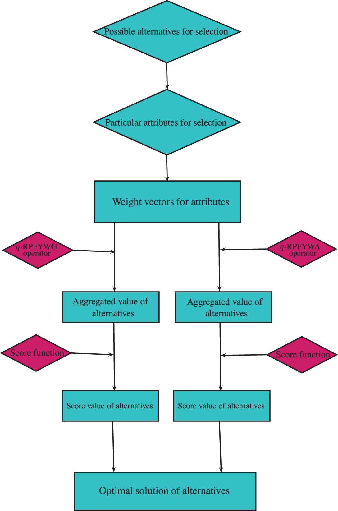
Framework for the selection of investment company.

6.3. Effect of Parameter ϑ on Decision-Making Results

To analyze the effect of parameter ϑ on results, we take distinct values of ϑ to handle the Application 6.1. The results for distinct values of ϑ for q-RPFYWA operator are shown in Table 3 and Figure 2, and for q-RPFYWG operator are shown in Table 4 and Figure 3.

ϑ S(g1) S(g2) S(g3) S(g4) RO
1 0.19 0.08 0.03 0.05 1>2>4>3
2 0.21 0.10 0.09 0.07 1>2>3>4
3 0.22 0.11 0.14 0.09 1>3>2>4
4 0.23 0.12 0.16 0.10 1>3>2>4
5 0.24 0.13 0.19 0.11 1>3>2>4
6 0.26 0.14 0.20 0.11 1>3>2>4
7 0.26 0.15 0.21 0.12 1>3>2>4
8 0.27 0.15 0.22 0.12 1>3>2>4
9 0.27 0.15 0.23 0.13 1>3>2>4
10 0.27 0.16 0.23 0.14 1>3>2>4
Table 3

Ranking order (RO) using q-rung picture fuzzy Yager weighted arithmetic (q-RPFYWA) operator.

Figure 2

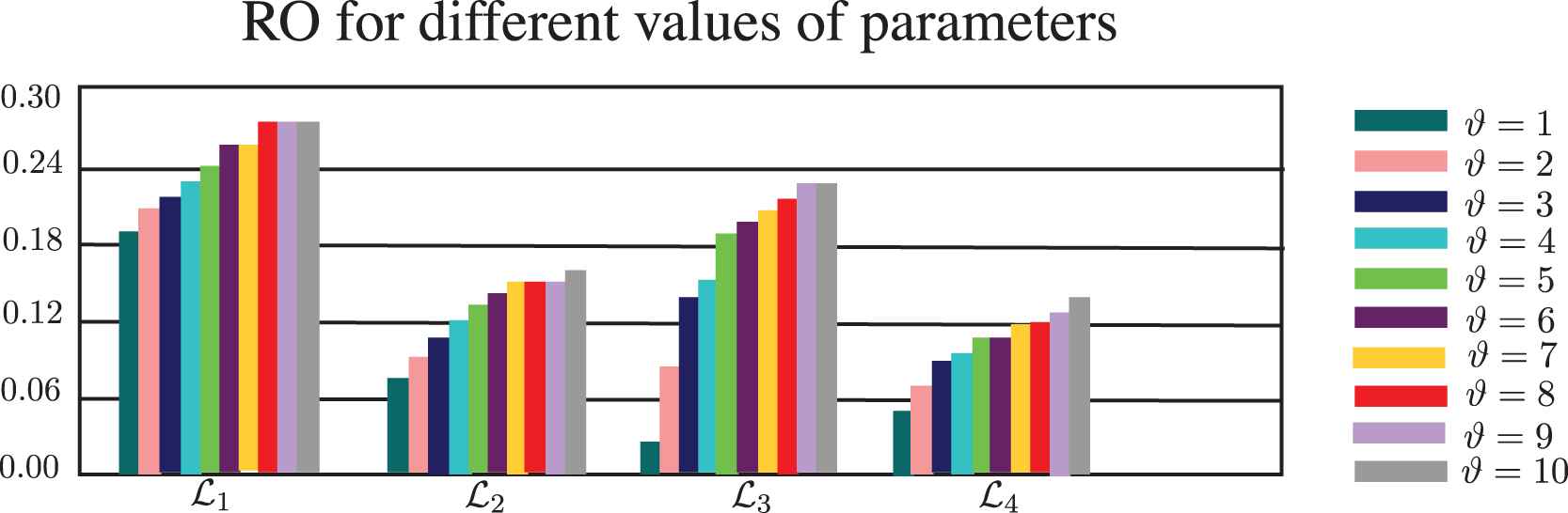
RO for different values of parameters using q-rung picture fuzzy Yager weighted arithmetic (-RPFYWA).

ϑ S(g1) S(g2) S(g3) S(g4) RO
1 0.19 0.08 0.03 0.05 1>2>4>3
2 0.19 0.08 0.01 0.04 1>2>4>3
3 0.17 0.07 −0.01 0.03 1>2>4>3
4 0.17 0.07 −0.03 0.01 1>2>4>3
5 0.15 0.06 −0.03 0.01 1>2>4>3
6 0.15 0.06 −0.04 0.01 1>2>4>3
7 0.15 0.06 −0.04 0.01 1>2>4>3
8 0.14 0.05 −0.04 −0.001 1>2>4>3
9 0.14 0.05 −0.05 −0.001 1>2>4>3
10 0.14 0.05 −0.06 −0.001 1>2>4>3
Table 4

RO using q-rung picture fuzzy Yager weighted arithmetic (q-RPFYWG) operator.

Figure 3

RO for different values of parameters using q-rung picture fuzzy Yager weighted arithmetic (-RPFYWG).

From above tables and figures, it can be seen that by taking various values of ϑ, the best alternative is same from both operators and best choice is 1. However, the overall ranking is slightly different. It is clear from Table 3 and Figure 2 that by using q-RPFYWA operator for ϑ=1,2, the ranking of alternatives is different and for ϑ=3,4,,10 the ranking is same. But for all values, 1 is the best. The score values of alternatives increase if value of ϑ increased. From Table 4 and Figure 3, it is clear that by using q-RPFYWG operator for ϑ=1,2,,10, the ranking of alternatives is same and best one is 1.

6.4. Comparison Analysis and Discussion

To compute performance and validity of our proposed operators, here we aggregate the same data using different operators, namely, picture fuzzy Einstein weighted average (PFEWA) [22], spherical fuzzy weighted average (SFWA) [7], spherical fuzzy weighted geometric (SFWG) [7] and picture fuzzy Dombi average (PFDWA) [20] operators. The computed results by applying these operators are summarized in Table 5 and shown in Figure 4.

Methods S(g1) S(g2) S(g3) S(g4) Ranking Order
q-RPFYWA 0.22 0.11 0.14 0.09 1>3>2>4
q-RPFYWG 0.17 0.07 −0.01 0.03 1>2>4>3
PFEWA 0.20 0.09 0.03 0.01 1>2>3>4
SFWA 0.20 0.09 0.06 0.01 1>2>3>4
SFWG 0.18 0.07 −0.03 0.04 1>2>4>3
PFDWA 0.22 0.10 0.05 0.04 1>2>3>4

q-RPFYWA, q-rung picture fuzzy Yager weighted arithmetic; PFEWA, picture fuzzy Einstein weighted average; SFWA, spherical fuzzy weighted average; SFWG, spherical fuzzy weighted geometric; PFDWA, picture fuzzy Dombi average.

Table 5

Comparison analysis with PFEWA, SFWA, SFWG and PFDWA operators (suppose q=3).

Figure 4

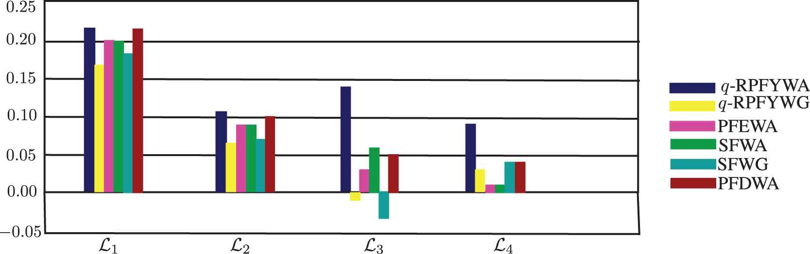
Comparison with existing operators.

It is clear from Table 5 and Figure 4 that best alternative obtained by using PFEWA, SFWA, SFWG and PFDWA operators remains same as obtained from proposed operators. This implies that our proposed methods are authentic and can be applied in DM problems. The main logic behind our proposed approach is that PFS and SFS handle the situations like μ+η+ν1 and μ2+η2+ν21, respectively but fail in situations where μq+ηq+νq1, where q3. That's why we need q-RPFS. The results from proposed theory are more accurate and closest to original results. However, in q-RPF Yager AOs, we can also discuss the effect of parameters.

7. CONCLUSIONS AND FUTURE DIRECTIONS

AOs are mathematical functions and imperative tools of unifying the many inputs into single valuable output. The q-RPFS, as a new generalization of PFS and SFS, allows to handle the situations with more generality than PFS and SFS, because it still works in the cases where μ+η+ν1 and μ2+η2+ν21 but it satisfies μq+ηq+νq1, where q3. Here, we have discussed MADM problems using q-RPF information. We have studied arithmetic and geometric operations to develop some q-RPF Yager AOs from the motivation of Yager operators as q-RPFYWA, q-RPFYOWA, q-RPFYHWA, q-RPFYWG, q-RPFYOWG and q-RPFYHWG operators. Different properties of these operators including idempotency, boundedness, monotonicity and reducibility are considered. Then, we have applied these operators to expand a few techniques to discuss MADM issues. Finally, practical example for emerging technology enterprise system selection is provided to develop a strategy. The proposed method is compared with the existing methods to show its advantages and appropriateness. Another example for the selection of a suitable company for investment under q-RPF data shows its importance. Moreover, we have discussed the DM results by taking distinct values of parameter. We will extend our work on the following DM problems:

  • An in-depth study of the Yager AOs for q-rung picture fuzzy information such as induced q-rung picture fuzzy Yager AOs, q-rung picture fuzzy Yager interactive AOs will be a hot topic in the future.

  • A MADM problem in medical diagnosis under q-rung picture fuzzy soft data using Yager AOs will be discussed.

  • A MADM problem for the selection of a smartphone under q-rung picture fuzzy soft data using Yager AOs will be discussed.

  • A robust DM model under m-polar fuzzy soft Yager AOs will be discussed.

CONFLICT OF INTEREST

The authors declare no conflicts of interest.

AUTHORS' CONTRIBUTIONS

Conceptualization, Muhammad Akram; Methodology, Peide Liu; Investigation, Gulfam Shahzadi. Writing—original Draft Preparation, Gulfam Shahzadi and Muhammad Akram; and Writing—review and Editing, Peide Liu.

ACKNOWLEDGMENTS

This paper is supported by the National Natural Science Foundation of China (No. 71771140), Project of cultural masters and “the four kinds of a batch” talents, the Special Funds of Taishan Scholars Project of Shandong Province (No. ts201511045), Major bidding projects of National Social Science Fund of China (19ZDA080).

REFERENCES

12.G. Deschrijver and E.E. Kerre, A generalization of operators on intuitionistic fuzzy sets using triangular norms and conorms, Notes Intuitionistic Fuzzy Sets, Vol. 8, 2002, pp. 19-27.
Journal
International Journal of Computational Intelligence Systems
Volume-Issue
13 - 1
Pages
1072 - 1091
Publication Date
2020/08/01
ISSN (Online)
1875-6883
ISSN (Print)
1875-6891
DOI
10.2991/ijcis.d.200717.001How to use a DOI?
Copyright
© 2020 The Authors. Published by Atlantis Press B.V.
Open Access
This is an open access article distributed under the CC BY-NC 4.0 license (http://creativecommons.org/licenses/by-nc/4.0/).

Cite this article

TY  - JOUR
AU  - Peide Liu
AU  - Gulfam Shahzadi
AU  - Muhammad Akram
PY  - 2020
DA  - 2020/08/01
TI  - Specific Types of q-Rung Picture Fuzzy Yager Aggregation Operators for Decision-Making
JO  - International Journal of Computational Intelligence Systems
SP  - 1072
EP  - 1091
VL  - 13
IS  - 1
SN  - 1875-6883
UR  - https://doi.org/10.2991/ijcis.d.200717.001
DO  - 10.2991/ijcis.d.200717.001
ID  - Liu2020
ER  -