
An Extreme Learning Machine and Gene Expression Programming-Based Hybrid Model for Daily Precipitation Prediction
- DOI
- 10.2991/ijcis.d.191126.001How to use a DOI?
- Keywords
- Extreme Learning Machine; Gene Expression Programming; Quantitative precipitation prediction; Rainfall prediction; Soft computing
- Abstract
Accurate daily precipitation prediction is crucially important. However, it is difficult to predict the precipitation accurately due to inherently complex meteorological factors and dynamic behavior of weather. Recently, considerable attention has been devoted in soft computing-based prediction approaches. This work presents a scheme to reduce the risk of Extreme Learning Machine (ELM) modeling error using Gene Expression Programming (GEP) to improve the prediction performance, and develops an ELM-GEP hybrid model for regional daily quantitative precipitation prediction. In this study, firstly, we use ELM for modeling the data sample of daily rainfall to construct a main model. Secondly, we use GEP for modeling the error of the main model as a compensation of the main model to reduce the prediction error. We conducted eight experiments of two different types of daily precipitation prediction problems using five metrics to evaluate our proposed model performance. Experimental results show that our model is comparable or even superior to five state-of-the-art models with high reliability in terms of all metrics on all datasets. It indicates that the proposed method is a promising alternative prediction tool for higher accuracy and credibility of regional daily precipitation prediction.
- Copyright
- © 2019 The Authors. Published by Atlantis Press SARL.
- Open Access
- This is an open access article distributed under the CC BY-NC 4.0 license (http://creativecommons.org/licenses/by-nc/4.0/).
1. INTRODUCTION
In modern times, weather forecasting plays an important role in human life. Accurate and timely precipitation prediction is crucial for our day-to-day activities and agriculture. And many business development plans also depend upon weather conditions. There is a huge loss of life and property due to the continuous or heavy rainfall and other unexpected rainfall conditions. Because they would lead to flood, mud-flows, rock-falls, landslides and other natural disasters or accidents. So, the accurate and efficient precipitation prediction also is of a great help for disaster prevention and water resources management, which must rely on rainfall forecasts to adjust the water volume of the reservoir for living water.
However, precipitation prediction is very complex and challenging. It is very difficult to model rainfall data using conventional linear and nonlinear approaches. Because a variety of inherently complicated factors, such as unknown climatic and geomorphological factors, are involved in the intricate hydro-logic micro-processes. Numerous researchers have attempted to improve the performance of the quantitative precipitation forecast (QPF) using various techniques, including: (1) numerical weather prediction (NWP) models and remote sensing observations [1–4], (2) statistical models [5–7] and (3) soft computing-based methods, such as artificial neural networks (ANNs) [8–10], support vector regression (SVR) [11–13], Extreme Learning Machine (ELM) [14,15], deep neural network (DNN) [16], fuzzy logic and others [17–21].
In recent years, soft computing-based machine learning methods have been widely utilized in combination with other methods to form the ensemble and conjunction methods, which are suggested as promising rainfall prediction methods [22–25]. Several examples of such methods will be mentioned. Ranjannayak [26] reviewed different techniques including Self Organizing Feature Maps Network, MultiLayer Perceptron Neural Network (MLP), Radial Basis Function Network (RBF), Back Propagation Neural Network (BP) and SVR, and concluded that most of the researchers used BP for rainfall prediction. Zhao et al. [27] designed a particle swarm optimization-neural network-based ensemble prediction model for typhoon rainstorm. The experimental results showed that their proposed model was more accurate than the NWP which was directly interpolated into the stations, indicating a potentially better operational weather prediction. Kim et al. [28] developed the hybrid models by combining neural computation, including support vector machines, generalized regression neural networks and wavelet technique for rainfall modeling. Their experiment results indicated that the combination of neural computing and wavelet technique can be a useful tool for modeling rainfall satisfactorily and can yield better efficiency than neural computing.
Daily quantitative precipitation prediction is more challenging in rainfall prediction in particular. Devi et al. [29] used different neural network models, such as Feed Forward BPk, Cascade Forward BP, Time delay neural network and Nonlinear Autoregressive Exogenous neural network (NARX), to predict rainfall one day in advance, and compared their forecasting capabilities. Dhar et al. [16] developed a DNN to achieve high performance and accuracy compared to the old conventional ways of forecasting the weather. Many studies about daily and short-range quantitative precipitation prediction in recent years have been focused on ensemble or conjunction methods based on soft computing methods coupled with other methods or NWP too. For example, Wu et al. [18] respectively integrated ANN and SVR coupled with Singular Spectrum Analysis and other data-preprocessing techniques to improve daily precipitation prediction. Unnikrishnan et al. [30] integrated SSA preprocessing algorithm in ANN models to enhance the performance of ANN models both in single and multi-time-step ahead daily rainfall prediction.
In brief, the literature indicates major disadvantages of current precipitation forecasts including: (1) There are various inherent and complex factors affecting rainfall, but it is difficult to find direct and effective predictors for prediction. (2) Because the scope of each grid represented the earth surface is relatively large, and the climate data in the analogue grid are shown as approximate average values. The climate predictions method based on NWP models and remote sensing observations models for larger-scale regions are more accurate, but it is difficult to segment the small-scale areas for forecasting rainfall [12]. (3) Because traditional mathematical and statistical methods are difficult to describe the nonlinear and nonstationary complex system of micro-meteorological processes, the accuracy and precision of mathematical and statistical-based methods are limited. (4) The forecast performance is difficult to meet the needs of people simply using soft computing-based methods due to the difficulties in describing the large-scale weather process and useless hydrological information. Therefore, in consideration of the importance of rainfall in our daily life and the difficulties to predict it, this work was to develop a precipitation prediction model based on ELM and Gene Expression Programming (GEP) to improve regional daily precipitation prediction.
ELM, proposed by Huang [31], not only learns much faster with higher generalization performance than the traditional gradient-based learning algorithms, but also learns network parameters analytically and avoids many difficulties faced by the gradient-based learning methods, such as stopping criteria, learning rate, learning epochs and local minimum [31]. ELM has been shown in many problems to achieve better performance than BP and support vector machine (SVM) in terms of learning speed, reliability and generalization [32].
GEP, proposed by Ferreira [33], is a very remarkable evolutionary algorithm, which inherits the advantages of Genetic Algorithms (GA) and Genetic Programming (GP) but gets rid of their shortcomings. GEP individuals are encoded as linear strings of fixed length which are afterwards expressed or translated into nonlinear entities of expression trees with different sizes and shapes. Its linear genotype and the constraint relations between head and tail of the chromosome make GEP run more efficiently and over 100–60000 times faster than GP [33]. These nonlinear entities are usually evolved into the sophisticated computer programs to solve a particular problem. Many researches show that GEP has very strong ability in data mining and optimization, and is especially suitable for dealing with function mining and symbolic regression problems [34,35].
The rest of the paper is organized as follows. Firstly, the related method theories are briefly introduced. Next, we clearly describes the proposed hybrid method. Then, we verify the feasibility and the advantages on performance of our model compared with the five state-of-the-art models for solving two different types of daily precipitation prediction problems. Finally, we conclude the work and suggest the future directions.
2. METHODS
In this section, related important theories which are useful for developing the proposed model are introduced, including ELM and GEP.
2.1. ELM basics
ELM is an effective single-hidden-layer feed forward neural networks (SLFNs) learning algorithm. It can obtain better generalization performance with the learning speed of thousands of times faster than that of the conventional feed forward network [31,36]. ELM, which is different from the traditional neural network learning algorithm, does not have to tune the hidden-layer but only needs to assign the number of hidden nodes of the network. The algorithm performance process is not necessary to adjust the input weights and the hidden element of bias [37], but only hunts for the optimal solution. Given
ELM aims to reach not only the smallest training error but also the smallest norm of output weights. According to Bartlett's theory, the smaller training error of the feed forward neural networks, the smaller norms of weights and the better generalization performance the networks tend to have. ELM randomly selects the input weights
The
The target function is continuous;
The input
If
Where
ELM can reach good generalization performance by ensuring two properties of learning: the smallest norm of weights and the smallest squared error on the training samples. But the gradient-based algorithms focus on the later property only. In general, the main procedure of the ELM can be generalized as follows:
Randomly assign the input weights
Calculate the hidden-layer output matrix
Calculate the output weight matrix
2.2. GEP Algorithm
GEP, which is based on the gene expression law of biological genetics, is regarded as the variant case with GP and GA. Generally, GEP has five components including terminal set, function set, control parameters, fitness function and stop condition. All of the five components need to be specified. GEP chromosome is represented by a fixed-length character string containing one or more genes. Each gene contains two parts: head and tail. The head can be composed of functions and terminals, while the tail can only consist of terminals. The function set is formed by all function symbols needed for solving the object problem while the terminals set consist of known symbols, variable and constant described the problem. And the relationship between the head length
Two expression forms of the chromosome of GEP are phenotype and genotype. Thus, each gene corresponds to a K-expression (the genotype of the chromosome) and an expression tree (the phenotype of the chromosome), which can be transformed into each other. As long as the expression tree is traversed from top to bottom and from left to right, it can be translated into K-expression. Similarly, as long as the symbols of K-expression are selected from left to right one by one and are filled layer by layer with new nodes of the expression tree consecutively, the K-expression can be translated into an expression tree. Furthermore, the chromosome structure was designed to enable the creation of multiple genes. Each gene is coded for a smaller program or sub-expression tree. When using GEP to solve a problem, the main algorithm description is similar with GP and GA, as shown in Figure 1.
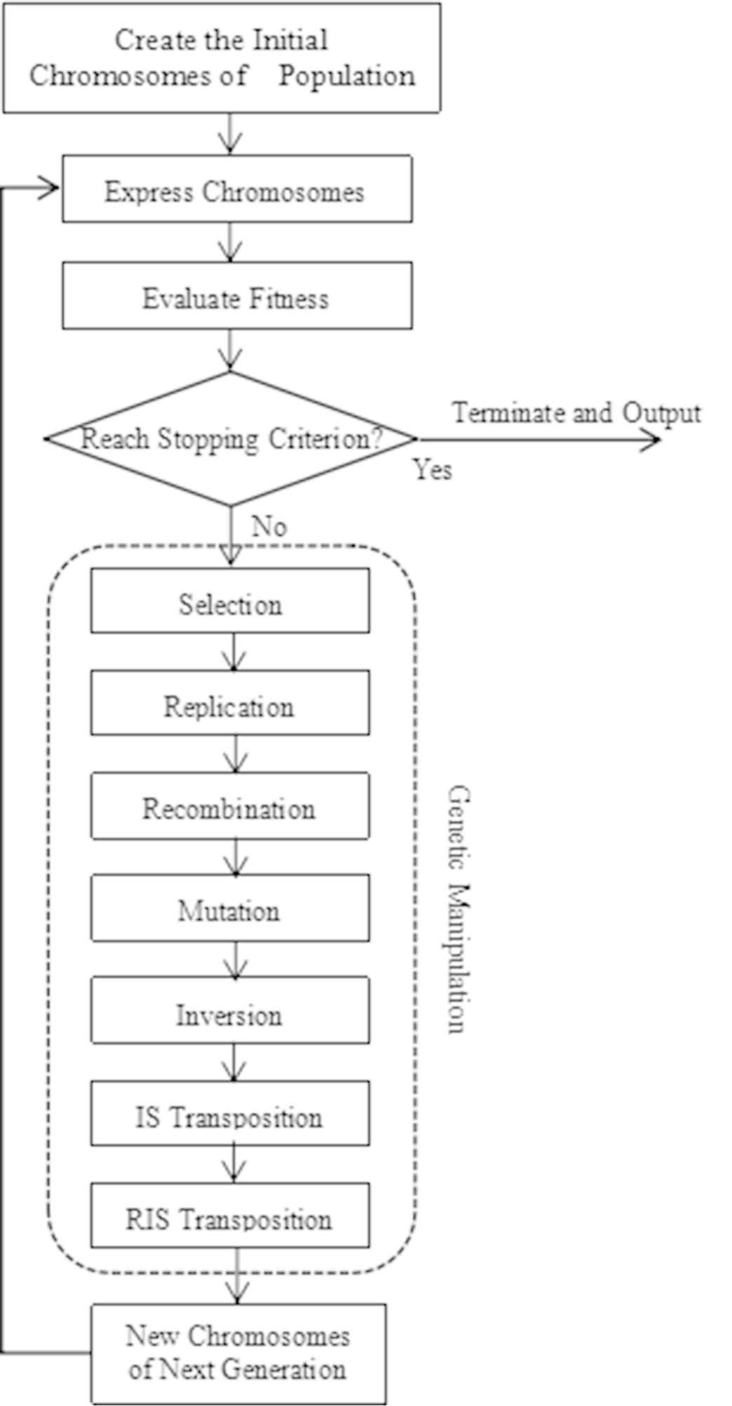
Flowchart of the Gene Expression Programming (GEP) algorithm.
3. PROPOSED METHODOLOGY
To summarize, the flowchart of the proposed hybrid modeling consists of three main steps drawn in blue background as shown in Figure 2. Firstly, precipitation-related datasets of the objective area is preprocessed by such data processing technologies as data normalization, feature selection and feature extraction. Secondly, the hybrid modeling method ELM-GEP is used to train the corresponding model. Finally, the trained model can be performed precipitation prediction, and its performance can be evaluated.
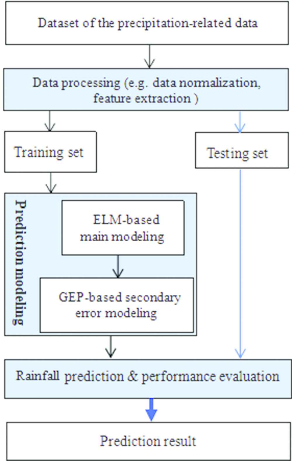
Main process flowchart of the proposed model.
3.1. Data Preprocessing
The quality of input data has a very important effect on data modeling. In order to improve the validity and accuracy of the model, some data-preprocessing works, including data cleaning and feature selection/extraction, should be done in accordance with specific problems and data before modeling.
3.2. The ELM-GEP Hybrid Modeling Algorithm
In General, the ELM well performs in processing large-size training samples benefiting from its parallel information processing configuration and high generalization performance. However, there may be a set of non-optimal or unnecessary input weights and hidden biases due to random selection only. It may lead to the output weights computed based on the input weights and the hidden biases being non-optimal. Thus the fitting ability and prediction performance are reduced. Therefore, ELM-GEP hybrid modeling method is proposed, whose main idea behind is to reduce the modeling error of ELM model to reach higher fitting ability and prediction performance. This hybrid model can be drawn as follows: Firstly, ELM is used for modeling the data samples of daily rainfall to construct a main model
So, the learning error of the ELM and GEP-based hybrid modeling on the data sample are given as:
Thus the optimization process of the proposed model is to minimize the
3.2.1. Modeling with ELM
In this study, ELM selected Sigmoid function as the activation function to model the data of daily rainfall. The number of input neurons was set by following the number of the meteorological properties, while the number of neurons in hidden-layers was set equal to the number of data conducted by literature [36]. It was only one neuron in output layer to represent the predicted precipitation. For example, to deal with the corresponding daily rainfall data containing 179 samples with 30 input variables, the basic schematic topological structure of the ELM network is constructed as shown in Figure 3.
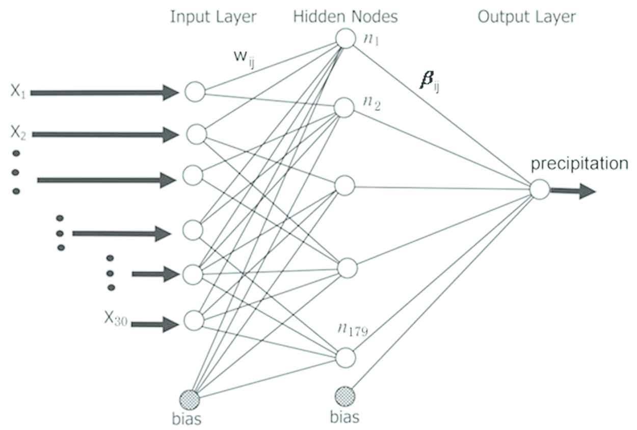
The topological structure of an Extreme Learning Machine network produced in this work. The input layer consists of 30 nodes, the hidden-layer contains 179 nodes, and the output layer has only one node that produces the predicted values of the daily precipitation.
3.2.2. Error modeling with GEP
The main ELM model has some errors that would affect the accuracy of fitting and prediction. In this paper, we use GEP to model the error of ELM to make up for rainfall prediction model. Our processing strategy is to calculate the errors between the sample value and the calculated value of the prediction model. Then, the error sequence is taken as a data sample for the error model builded by GEP. Finally, the error model is compensated to the prediction model. The algorithm would automatically calculate the sample value prediction error between computed value and compensation again, until the fitness value of GEP is up to the predefined stopping criterion. And it is taken as sample data to modeling by GEP, what would compensate for the prediction model. Do this process again until it meets the requirements.
3.2.3. The ELM-GEP algorithm
The flowchart of the ELM-GEP algorithm is given in Figure 4. ELM-GEP algorithm process contains three phases, whose main steps involved are summarized as follows:
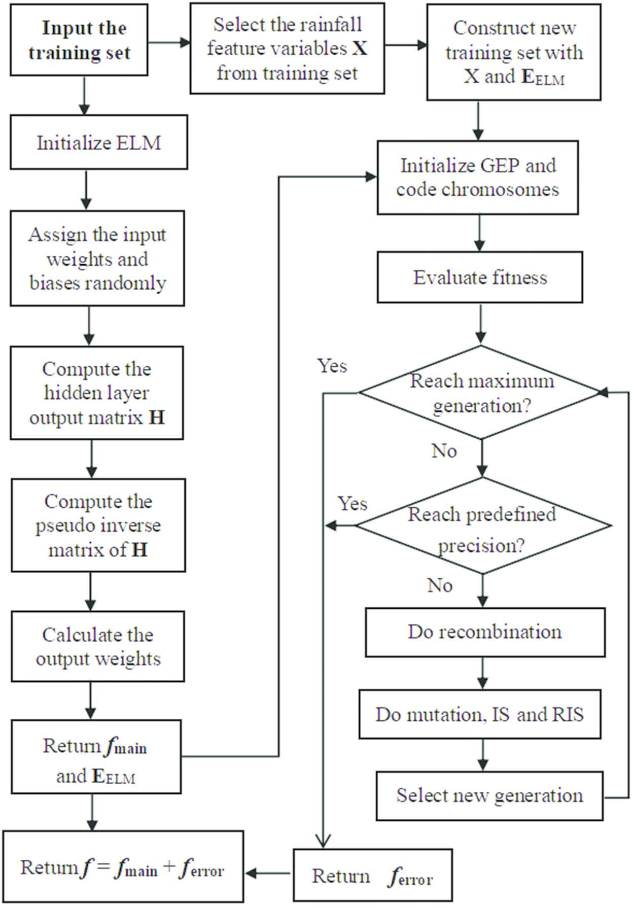
Flowchart of the Extreme Learning Machine (ELM)-Gene Expression Programming (GEP) precipitation prediction algorithm.
Phase 1 (main modeling phase): Input the training set of daily rainfall, then build the main model by ELM.
Generate the input weights and biases randomly;
Calculate the hidden-layer output matrix
Calculate the pseudo-inverse matrix;
Set the output weights;
Return the main model
Phase 2 (error modeling phase): Input the
Input the
Initialize GEP algorithm, and code chromosomes with new training set;
Evaluate fitness;
Select chromosomes;
Do recombination;
Do mutation, insertion sequence (IS) and root insertion sequence (RIS);
Evaluate fitness;
Loop (4) of the Phase 2 unless the maximum generation is reached;
If achieve the predefined precision, then return the decoding result of the best chromosome as the error model
Phase 3: Construct the ELM-GEP hybrid prediction model
4. EXPERIMENT
In this study, eight real-world datasets are used to evaluate the proposed method by two different types of daily precipitation prediction problems, including the daily precipitation prediction of 48 hours in advance and on the current day. These eight datasets contain three Guangxi datasets [22], two southwestern India datasets [16] and three Chittagong datasets that are available in https://github.com/TanvirMahmudEmon.
4.1. Experimental Setup
4.1.1. Performance measurement
The performance of our method is evaluated by five metrics including mean absolute error (MAE), root mean square error (RMSE), Pearson Relative Coefficient (PRC), Strong Credible Prediction Ratio (SC Ratio) and Unbelievable Prediction Ratio (UB Ratio). SC Ratio is defined as
4.1.2. Comparison methods and parameters setting
To verify the advantage of our model, we evaluated ELM-GEP against five state-of-the-art methods, including DNN, ELM, SVR, BP and NARX. The main parameters setting of these algorithms in this work are listed in Table 1, where the parameters of GEP and DNN follow the setting in the literatures [34] and [16], respectively. The other parameters of these algorithms are tuned by Grid Search method using the daily rainfall data in July of zone 3. In order to avoid a biased algorithmic setup caused by parameter tuning, this dataset will not be used for comparative experiments.
| Algorithm | Parameter | Value |
|---|---|---|
| GEP | Popular size | 100 |
| Head length | 17 | |
| Function set | +, −, *, /, sin, cos | |
| Maximum generation | 1000 | |
| Fitness function | 1/RMSE | |
| 1/2-point cross rate | 0.3 | |
| Mutation rate | 0.3 | |
| IS/RIS rate | 0.03 | |
| Inversion rate | 0.03 | |
| ELM | Activation function | Gaussian function |
| Kernel function | RBF | |
| Number of hidden neurons | 148 | |
| Number of hidden-layers | 1 | |
| Regularization coefficient | 0.9 | |
| DNN | Activation function | Relu function |
| optimizer | Adam | |
| Number of hidden-layers | 6 | |
| Number of hidden neurons | [100, 95, 105, 98, 102, 100] | |
| Batch-size | 15 | |
| Epochs | 1000 | |
| SVR | Kernel function | RBF |
| Epsilon | 0.005 | |
| Gamma | 0.01 | |
| SVM-type | Epsilon SVR | |
| BP | Activation function | Sigmoid |
| Epochs | 1000 | |
| Number of hidden neurons | 148 | |
| Number of hidden-layers | 3 | |
| Lr | 0.0015 | |
| NARX | Activation function | Gaussian function |
| Number of hidden neurons | 148 | |
| Number of hidden-layers | 3 | |
| Timedelay | 1:2 | |
| TrainRatio | 0.167 |
GEP, Gene Expression Programming; ELM, Extreme Learning Machine; DNN, deep neural network; SVR, Support Vector Regression; BP, Back Propagation Neural Network; NARX, Nonlinear Autoregressive Exogenous neural network; RMSE, root mean square error; RBF, Radial Basis Function Network.
Main parameters of algorithms in the study.
Because the task of the 48-hour ahead daily rainfall prediction requires time continuity and sequentiality of data samples, it is not conducive to cross-validation of Guangxi datasets experiment, so we conducted some t-tests on holdout validation to validate the performance of various models. The data samples from 2003 to 2007 of the Guangxi datasets were used for model training, and the remains of them were used for prediction test. The task of the precipitation prediction on the current day does not need time continuity and sequentiality of data samples. Therefore, we conducted some t-tests on 5-fold cross-validation for the precipitation prediction on the current day on the datasets of Chittagong and southwestern India.
All the results presented in this paper are the mean values of 50 independent runs of the corresponding model on the same testing dataset to avoid stochastic deviation. Note that in all the experimental results tables (Tables 2–6), the third and the fourth columns are the mean and standard deviation of the MAE score respectively, and the sixth and seventh columns are the mean and standard deviation of the RMSE score respectively. The fifth and eighth columns are the P-values of t-test comparisons between our proposed model and the other comparing models in terms of MAE and RMSE, respectively.
| Dataset | Models | MAE |
RMSE |
PRC | SC Ratio | UB Ratio | ||||
|---|---|---|---|---|---|---|---|---|---|---|
| mAve | mStd | mP-value | rAve | rStd | rP-value | |||||
| India-7 | ELM-GEP | 4.009 | 1.010 | 7.112 | 4.030 | 0.766 | 0.806 | 0.080 | ||
| DNN | 4.673 | 2.235 | 0.058 | 8.714 | 4.485 | 0.070 | 0.757 | 0.664 | 0.143 | |
| ELM | 4.612 | 2.004 | 0.060 | 10.408 | 4.040 | 0.000 | 0.763 | 0.803 | 0.147 | |
| SVM | 4.360 | 3.555 | 0.496 | 11.284 | 5.880 | 0.000 | 0.763 | 0.806 | 0.139 | |
| BP | 6.104 | 2.324 | 0.000 | 10.619 | 5.478 | 0.001 | 0.714 | 0.322 | 0.113 | |
| NARX | 6.302 | 2.044 | 0.000 | 10.265 | 5.317 | 0.001 | 0.717 | 0.462 | 0.144 | |
| India-8 | ELM-GEP | 4.008 | 1.011 | 7.812 | 4.015 | 0.776 | 0.815 | 0.080 | ||
| DNN | 5.313 | 2.302 | 0.000 | 9.508 | 4.893 | 0.067 | 0.757 | 0.594 | 0.144 | |
| ELM | 4.361 | 2.001 | 0.274 | 10.408 | 5.401 | 0.043 | 0.773 | 0.813 | 0.136 | |
| SVM | 4.354 | 3.533 | 0.509 | 11.231 | 5.853 | 0.001 | 0.762 | 0.808 | 0.136 | |
| BP | 6.134 | 2.263 | 0.000 | 10.527 | 5.422 | 0.006 | 0.714 | 0.284 | 0.112 | |
| NARX | 6.661 | 2.162 | 0.000 | 10.838 | 5.637 | 0.003 | 0.707 | 0.454 | 0.156 | |
MAE, mean absolute error; RMSE, root mean square error; PRC, Pearson Relative Coefficient; SC, Strong Credible Prediction Ratio; UB, Unbelievable Prediction Ratio; ELM, Extreme Learning Machine; GEP, Gene Expression Programming; DNN, deep neural network; BP, Back Propagation Neural Network; NARX, Nonlinear Autoregressive Exogenous neural network.
Note: The best results of each metric on the dataset India-7 and India-8 are highlighted by blue and yellow, respectively.
The comparison results on the southwestern India datasets.
| Dataset | Models | MAE |
RMSE |
PRC | SC Ratio | UB Ratio | ||||
|---|---|---|---|---|---|---|---|---|---|---|
| mAve | mStd | mP-value | rAve | rStd | rP-value | |||||
| Chit-6 | ELM-GEP | 0.023 | 0.002 | 0.105 | 0.010 | 0.957 | 1.000 | 0.000 | ||
| DNN | 0.029 | 0.009 | 0.000 | 0.090 | 0.035 | 0.005 | 0.957 | 1.000 | 0.000 | |
| ELM | 0.031 | 0.009 | 0.000 | 0.132 | 0.011 | 0.000 | 0.933 | 1.000 | 0.000 | |
| SVM | 0.024 | 0.000 | 0.010 | 0.109 | 0.007 | 0.028 | 0.949 | 1.000 | 0.000 | |
| BP | 0.075 | 0.012 | 0.000 | 0.141 | 0.016 | 0.000 | 0.924 | 1.000 | 0.000 | |
| NARX | 0.038 | 0.004 | 0.000 | 0.144 | 0.015 | 0.000 | 0.927 | 1.000 | 0.000 | |
| Chit-7 | ELM-GEP | 0.096 | 0.008 | 0.402 | 0.018 | 0.956 | 0.996 | 0.003 | ||
| DNN | 0.117 | 0.044 | 0.001 | 0.447 | 0.211 | 0.136 | 0.955 | 0.996 | 0.003 | |
| ELM | 0.121 | 0.024 | 0.000 | 0.589 | 0.016 | 0.000 | 0.953 | 0.995 | 0.005 | |
| SVM | 0.098 | 0.001 | 0.099 | 0.554 | 0.024 | 0.000 | 0.956 | 0.995 | 0.005 | |
| BP | 0.185 | 0.029 | 0.000 | 0.599 | 0.016 | 0.000 | 0.950 | 0.995 | 0.005 | |
| NARX | 0.158 | 0.030 | 0.000 | 0.747 | 0.103 | 0.000 | 0.947 | 0.987 | 0.005 | |
| Chit-8 | ELM-GEP | 0.071 | 0.010 | 0.192 | 0.028 | 0.967 | 1.000 | 0.000 | ||
| DNN | 0.066 | 0.059 | 0.557 | 0.252 | 0.227 | 0.067 | 0.967 | 0.998 | 0.002 | |
| ELM | 0.112 | 0.014 | 0.000 | 0.602 | 0.041 | 0.000 | 0.913 | 0.995 | 0.005 | |
| SVM | 0.098 | 0.001 | 0.000 | 0.543 | 0.031 | 0.000 | 0.912 | 0.995 | 0.005 | |
| BP | 0.168 | 0.020 | 0.000 | 0.566 | 0.026 | 0.000 | 0.914 | 0.995 | 0.005 | |
| NARX | 0.202 | 0.028 | 0.000 | 0.848 | 0.091 | 0.000 | 0.917 | 0.987 | 0.005 | |
MAE, mean absolute error; RMSE, root mean square error; PRC, Pearson Relative Coefficient; SC, Strong Credible Prediction Ratio; UB, Unbelievable Prediction Ratio; ELM, Extreme Learning Machine; GEP, Gene Expression Programming; DNN, deep neural network; BP, Back Propagation Neural Network; NARX, Nonlinear Autoregressive Exogenous neural network.
Note: The best results of each metric on the Chit-6, Chit-7 and Chit-8 are highlighted by blue, yellow and gray, respectively.
The comparison results on the Chittagong datasets.
| Zone | Models | MAE |
RMSE |
PRC | SC Ratio | UB Ratio | ||||
|---|---|---|---|---|---|---|---|---|---|---|
| mAve | mStd | mP-value | rAve | rStd | rP-value | |||||
| 1 | ELM-GEP+ | 4.530 | 0.251 | 6.982 | 0.323 | 0.851 | 0.800 | 0.033 | ||
| ELM+ | 4.664 | 0.316 | 0.022 | 7.572 | 0.328 | 0.000 | 0.786 | 0.667 | 0.167 | |
| SVM+ | 4.593 | 0.000 | 0.082 | 9.112 | 0.000 | 0.000 | 0.803 | 0.733 | 0.133 | |
| BP+ | 4.702 | 0.322 | 0.004 | 8.925 | 0.332 | 0.000 | 0.776 | 0.633 | 0.200 | |
| NARX+ | 5.175 | 0.419 | 0.000 | 7.389 | 0.329 | 0.000 | 0.767 | 0.567 | 0.167 | |
| DNN | 4.698 | 0.543 | 0.052 | 7.783 | 0.611 | 0.000 | 0.779 | 0.767 | 0.067 | |
| ELM-GEP | 5.275 | 0.321 | 0.000 | 7.855 | 0.351 | 0.000 | 0.757 | 0.533 | 0.167 | |
| ELM | 5.923 | 0.387 | 0.000 | 7.774 | 0.343 | 0.000 | 0.748 | 0.533 | 0.133 | |
| SVM | 7.110 | 0.000 | 0.000 | 11.214 | 0.000 | 0.000 | 0.685 | 0.467 | 0.233 | |
| BP | 7.494 | 0.405 | 0.000 | 11.501 | 0.340 | 0.000 | 0.679 | 0.367 | 0.233 | |
| NARX | 5.464 | 0.413 | 0.000 | 7.572 | 0.337 | 0.000 | 0.756 | 0.467 | 0.167 | |
| 2 | ELM-GEP+ | 4.491 | 0.258 | 7.378 | 0.357 | 0.838 | 0.800 | 0.067 | ||
| ELM+ | 4.628 | 0.282 | 0.014 | 9.378 | 0.371 | 0.000 | 0.773 | 0.767 | 0.100 | |
| SVM+ | 4.617 | 0.000 | 0.001 | 9.227 | 0.000 | 0.000 | 0.802 | 0.767 | 0.067 | |
| BP+ | 4.987 | 0.337 | 0.000 | 9.006 | 0.369 | 0.000 | 0.774 | 0.567 | 0.133 | |
| NARX+ | 5.246 | 0.366 | 0.000 | 9.007 | 0.375 | 0.000 | 0.739 | 0.533 | 0.167 | |
| DNN | 5.051 | 0.562 | 0.000 | 8.469 | 0.618 | 0.000 | 0.767 | 0.633 | 0.067 | |
| ELM-GEP | 5.706 | 0.313 | 0.000 | 8.890 | 0.369 | 0.000 | 0.723 | 0.433 | 0.167 | |
| ELM | 6.286 | 0.324 | 0.000 | 8.749 | 0.377 | 0.000 | 0.706 | 0.233 | 0.100 | |
| SVM | 6.189 | 0.000 | 0.000 | 10.570 | 0.000 | 0.000 | 0.707 | 0.500 | 0.167 | |
| BP | 6.377 | 0.327 | 0.000 | 10.569 | 0.385 | 0.000 | 0.705 | 0.433 | 0.133 | |
| NARX | 6.105 | 0.319 | 0.000 | 8.799 | 0.399 | 0.000 | 0.701 | 0.267 | 0.133 | |
| 3 | ELM-GEP+ | 3.809 | 0.239 | 7.061 | 0.295 | 0.847 | 0.867 | 0.067 | ||
| ELM+ | 3.907 | 0.288 | 0.070 | 8.033 | 0.315 | 0.000 | 0.818 | 0.733 | 0.100 | |
| SVM+ | 3.992 | 0.000 | 0.002 | 8.669 | 0.000 | 0.000 | 0.816 | 0.767 | 0.100 | |
| BP+ | 4.241 | 0.267 | 0.000 | 8.441 | 0.322 | 0.000 | 0.788 | 0.633 | 0.100 | |
| NARX+ | 4.623 | 0.302 | 0.000 | 7.840 | 0.336 | 0.000 | 0.772 | 0.567 | 0.167 | |
| DNN | 4.332 | 0.488 | 0.000 | 8.131 | 0.587 | 0.000 | 0.781 | 0.667 | 0.067 | |
| ELM-GEP | 5.415 | 0.296 | 0.000 | 8.215 | 0.323 | 0.000 | 0.735 | 0.467 | 0.167 | |
| ELM | 6.084 | 0.309 | 0.000 | 8.162 | 0.328 | 0.000 | 0.720 | 0.233 | 0.167 | |
| SVM | 5.575 | 0.000 | 0.000 | 9.517 | 0.000 | 0.000 | 0.721 | 0.633 | 0.167 | |
| BP | 5.914 | 0.311 | 0.000 | 9.173 | 0.331 | 0.000 | 0.713 | 0.367 | 0.133 | |
| NARX | 5.550 | 0.325 | 0.000 | 7.918 | 0.359 | 0.000 | 0.752 | 0.400 | 0.133 | |
MAE, mean absolute error; RMSE, root mean square error; PRC, Pearson Relative Coefficient; SC, Strong Credible Prediction Ratio; UB, Unbelievable Prediction Ratio; ELM, Extreme Learning Machine; GEP, Gene Expression Programming; DNN, deep neural network; BP, Back Propagation Neural Network; NARX, Nonlinear Autoregressive Exogenous neural network. Note: The best results of each metric on the zone 1, zone 2 and zone 3 are highlighted by blue, yellow and gray, respectively.
The comparison results on the Guang-4 dataset.
| Zone | Models | MAE |
RMSE |
PRC | SC Ratio | UB Ratio | ||||
|---|---|---|---|---|---|---|---|---|---|---|
| mAve | mStd | mP-value | rAve | rStd | rP-value | |||||
| 1 | ELM-GEP+ | 4.308 | 0.221 | 5.218 | 0.619 | 0.731 | 0.806 | 0.065 | ||
| ELM+ | 4.650 | 0.238 | 0.000 | 8.969 | 0.662 | 0.000 | 0.718 | 0.452 | 0.065 | |
| SVM+ | 5.209 | 0.000 | 0.000 | 8.265 | 0.000 | 0.000 | 0.719 | 0.516 | 0.097 | |
| BP+ | 6.072 | 0.242 | 0.000 | 9.917 | 0.639 | 0.000 | 0.667 | 0.419 | 0.194 | |
| NARX+ | 6.751 | 0.488 | 0.000 | 15.839 | 1.311 | 0.000 | 0.633 | 0.419 | 0.258 | |
| DNN | 4.448 | 0.537 | 0.095 | 6.256 | 0.932 | 0.000 | 0.729 | 0.774 | 0.065 | |
| ELM-GEP | 7.718 | 0.269 | 0.000 | 11.408 | 0.799 | 0.000 | 0.663 | 0.323 | 0.226 | |
| ELM | 7.933 | 0.282 | 0.000 | 13.011 | 0.826 | 0.000 | 0.662 | 0.323 | 0.194 | |
| SVM | 7.838 | 0.000 | 0.000 | 12.338 | 0.000 | 0.000 | 0.657 | 0.323 | 0.226 | |
| BP | 7.543 | 0.257 | 0.000 | 15.722 | 0.942 | 0.000 | 0.661 | 0.323 | 0.129 | |
| NARX | 7.355 | 0.620 | 0.000 | 11.104 | 0.659 | 0.000 | 0.627 | 0.387 | 0.258 | |
| 2 | ELM-GEP+ | 3.008 | 0.175 | 3.800 | 0.387 | 0.867 | 0.806 | 0.000 | ||
| ELM+ | 3.422 | 0.172 | 0.000 | 7.378 | 0.394 | 0.000 | 0.790 | 0.677 | 0.097 | |
| SVM+ | 3.020 | 0.000 | 0.632 | 5.837 | 0.000 | 0.000 | 0.817 | 0.806 | 0.000 | |
| BP+ | 4.841 | 0.146 | 0.000 | 8.354 | 0.615 | 0.000 | 0.748 | 0.581 | 0.129 | |
| NARX+ | 4.396 | 0.178 | 0.000 | 7.837 | 0.507 | 0.000 | 0.712 | 0.516 | 0.226 | |
| DNN | 3.321 | 0.689 | 0.000 | 4.873 | 1.105 | 0.000 | 0.848 | 0.806 | 0.032 | |
| ELM-GEP | 5.158 | 0.125 | 0.000 | 10.067 | 0.508 | 0.000 | 0.687 | 0.452 | 0.161 | |
| ELM | 5.404 | 0.138 | 0.000 | 10.800 | 0.567 | 0.000 | 0.665 | 0.387 | 0.097 | |
| SVM | 5.256 | 0.000 | 0.000 | 10.097 | 0.000 | 0.000 | 0.687 | 0.452 | 0.161 | |
| BP | 5.048 | 0.151 | 0.000 | 10.140 | 0.556 | 0.000 | 0.688 | 0.484 | 0.129 | |
| NARX | 5.130 | 0.188 | 0.000 | 7.872 | 0.593 | 0.000 | 0.707 | 0.484 | 0.097 | |
| 3 | ELM-GEP+ | 2.913 | 0.169 | 3.396 | 0.152 | 0.902 | 0.871 | 0.000 | ||
| ELM+ | 3.347 | 0.412 | 0.000 | 4.338 | 0.165 | 0.000 | 0.841 | 0.677 | 0.097 | |
| SVM+ | 3.198 | 0.000 | 0.000 | 5.077 | 0.000 | 0.000 | 0.782 | 0.677 | 0.032 | |
| BP+ | 4.764 | 0.389 | 0.000 | 8.179 | 0.187 | 0.000 | 0.758 | 0.613 | 0.097 | |
| NARX+ | 5.067 | 0.418 | 0.000 | 8.364 | 0.506 | 0.000 | 0.742 | 0.548 | 0.258 | |
| DNN | 3.296 | 0.781 | 0.000 | 4.730 | 1.149 | 0.000 | 0.862 | 0.806 | 0.032 | |
| ELM-GEP | 6.942 | 0.506 | 0.000 | 9.884 | 0.527 | 0.000 | 0.690 | 0.484 | 0.129 | |
| ELM | 7.353 | 0.543 | 0.000 | 10.719 | 0.795 | 0.000 | 0.687 | 0.452 | 0.129 | |
| SVM | 7.227 | 0.000 | 0.000 | 9.868 | 0.000 | 0.000 | 0.708 | 0.484 | 0.129 | |
| BP | 6.848 | 0.620 | 0.000 | 11.405 | 0.996 | 0.000 | 0.692 | 0.387 | 0.129 | |
| NARX | 6.684 | 0.632 | 0.000 | 7.684 | 0.593 | 0.000 | 0.717 | 0.516 | 0.097 | |
MAE, mean absolute error; RMSE, root mean square error; PRC, Pearson Relative Coefficient; SC, Strong Credible Prediction Ratio; UB, Unbelievable Prediction Ratio; ELM, Extreme Learning Machine; GEP, Gene Expression Programming; DNN, deep neural network; BP, Back Propagation Neural Network; NARX, Nonlinear Autoregressive Exogenous neural network.
Note: The best results of each metric on the zone 1, zone 2 and zone 3 are highlighted by blue, yellow and gray, respectively.
The comparison results on the Guang-5 dataset.
| Zone | Models | MAE | RMSE | PRC | SC Ratio | UB Ratio | ||||
|---|---|---|---|---|---|---|---|---|---|---|
| mAve | mStd | mP-value | rAve | rStd | rP-value | |||||
| 1 | ELM-GEP+ | 6.719 | 0.209 | 11.812 | 0.868 | 0.646 | 0.533 | 0.167 | ||
| ELM+ | 6.837 | 0.306 | 0.028 | 14.338 | 1.001 | 0.000 | 0.638 | 0.500 | 0.200 | |
| SVM+ | 6.806 | 0.000 | 0.004 | 14.314 | 0.000 | 0.000 | 0.639 | 0.500 | 0.200 | |
| BP+ | 7.002 | 0.413 | 0.000 | 16.242 | 1.112 | 0.000 | 0.627 | 0.500 | 0.233 | |
| NARX+ | 7.015 | 0.389 | 0.000 | 18.839 | 1.125 | 0.000 | 0.625 | 0.400 | 0.233 | |
| DNN | 6.933 | 0.557 | 0.013 | 12.405 | 0.867 | 0.000 | 0.642 | 0.533 | 0.200 | |
| ELM-GEP | 7.611 | 0.350 | 0.000 | 18.408 | 1.206 | 0.000 | 0.613 | 0.333 | 0.200 | |
| ELM | 7.763 | 0.375 | 0.000 | 20.011 | 1.558 | 0.000 | 0.610 | 0.333 | 0.233 | |
| SVM | 7.658 | 0.000 | 0.000 | 19.338 | 0.000 | 0.000 | 0.612 | 0.333 | 0.233 | |
| BP | 7.443 | 0.248 | 0.000 | 21.722 | 1.501 | 0.000 | 0.614 | 0.333 | 0.267 | |
| NARX | 7.055 | 0.508 | 0.000 | 17.104 | 0.788 | 0.000 | 0.617 | 0.400 | 0.233 | |
| 2 | ELM-GEP+ | 3.951 | 0.226 | 10.065 | 0.699 | 0.782 | 0.767 | 0.100 | ||
| ELM+ | 4.042 | 0.301 | 0.094 | 13.873 | 0.752 | 0.000 | 0.770 | 0.767 | 0.133 | |
| SVM+ | 4.034 | 0.000 | 0.012 | 12.877 | 0.000 | 0.000 | 0.772 | 0.567 | 0.167 | |
| BP+ | 4.078 | 0.381 | 0.048 | 15.042 | 1.006 | 0.000 | 0.768 | 0.367 | 0.167 | |
| NARX+ | 4.082 | 0.403 | 0.050 | 13.361 | 0.859 | 0.000 | 0.766 | 0.567 | 0.167 | |
| DNN | 4.202 | 0.650 | 0.012 | 10.878 | 0.926 | 0.000 | 0.778 | 0.767 | 0.133 | |
| ELM-GEP | 4.369 | 0.433 | 0.000 | 13.067 | 0.822 | 0.000 | 0.757 | 0.467 | 0.167 | |
| ELM | 4.504 | 0.451 | 0.000 | 15.800 | 0.813 | 0.000 | 0.750 | 0.400 | 0.167 | |
| SVM | 4.386 | 0.000 | 0.000 | 14.097 | 0.000 | 0.000 | 0.755 | 0.467 | 0.167 | |
| BP | 4.348 | 0.920 | 0.000 | 20.140 | 1.001 | 0.000 | 0.758 | 0.500 | 0.233 | |
| NARX | 4.090 | 0.525 | 0.092 | 12.872 | 0.567 | 0.000 | 0.765 | 0.467 | 0.200 | |
| 3 | ELM-GEP+ | 4.059 | 0.401 | 10.946 | 0.402 | 0.761 | 0.800 | 0.133 | ||
| ELM+ | 4.833 | 0.368 | 0.000 | 11.122 | 0.423 | 0.037 | 0.733 | 0.567 | 0.167 | |
| SVM+ | 4.808 | 0.000 | 0.000 | 12.988 | 0.000 | 0.000 | 0.739 | 0.567 | 0.133 | |
| BP+ | 5.090 | 0.411 | 0.000 | 19.014 | 1.414 | 0.000 | 0.717 | 0.367 | 0.200 | |
| NARX+ | 5.171 | 0.607 | 0.000 | 12.786 | 0.875 | 0.000 | 0.708 | 0.533 | 0.200 | |
| DNN | 4.711 | 0.502 | 0.000 | 11.621 | 0.690 | 0.000 | 0.751 | 0.767 | 0.133 | |
| ELM-GEP | 6.182 | 0.513 | 0.000 | 17.884 | 1.007 | 0.000 | 0.660 | 0.500 | 0.200 | |
| ELM | 7.053 | 0.527 | 0.000 | 18.019 | 1.021 | 0.000 | 0.617 | 0.467 | 0.200 | |
| SVM | 6.727 | 0.000 | 0.000 | 17.868 | 0.000 | 0.000 | 0.642 | 0.500 | 0.233 | |
| BP | 5.948 | 0.366 | 0.000 | 18.405 | 1.433 | 0.000 | 0.664 | 0.533 | 0.233 | |
| NARX | 5.684 | 0.398 | 0.000 | 15.684 | 0.998 | 0.000 | 0.687 | 0.500 | 0.200 | |
MAE, mean absolute error; RMSE, root mean square error; PRC, Pearson Relative Coefficient; SC, Strong Credible Prediction Ratio; UB, Unbelievable Prediction Ratio; ELM, Extreme Learning Machine; GEP, Gene Expression Programming; DNN, deep neural network; BP, Back Propagation Neural Network; NARX, Nonlinear Autoregressive Exogenous neural network.
Note: The best results of each metric on the zone 1, zone 2 and zone 3 are highlighted by blue, yellow and gray, respectively.
The comparison results on the Guang-6 dataset.
4.2. The Precipitation Prediction on the Current Day
In this section, we conducted five cases of the precipitation prediction on the current day to verify our model.
4.2.1. The study of predicting area and data
The southwestern India has a tropical monsoon climate of monsoon rainy seasons from June to September. It is generally difficult to accurately predict the precipitation in southwestern India, as this area is characterized by complicated topography with starkly different microclimates.
There are July dataset (called India-7) and August dataset (called India-8) collected by the Indian Statistical Institute, which was used in the literature [16]. These two datasets are daily precipitation data of a state in southwestern India from 1989 to 1995 with 8 available characteristic attributes affecting precipitation. There are 216 and 214 precipitation data samples in India-7 and India-8 dataset, respectively.
Chittagong is the largest port city in Bangladesh located on the northeastern shore of the Bay of Bengal. Chittagong has a tropical monsoon climate, which hosts a monsoon rainy season from June to August. Datasets of Chittagong are daily precipitation datasets of June, July and August from 2012 to 2017 (hereafter called Chit-6, Chit-7 and Chit-8 dataset, respectively) with 17 available characteristic attributes affecting precipitation. Chit-6, Chit-7 and Chit-8 datasets contain 180, 186 and 186 precipitation data samples, respectively.
4.2.2. Data preprocessing for the datasets of Southwestern India and Chittagong
The original datasets of southwestern India and Chittagong have 10 and 17 available selected characteristic attributes affecting rainfall except for the time attributes, respectively. These datasets had been conducted preliminary data cleaning and feature screening by the dataset collectors. Therefore, in this work, we only conducted data normalization using Z-Score and missing value dealing, did not extract feature to utilize more information of attributes.
4.2.3. Performance evaluation of the precipitation prediction on the current day
In this section, we demonstrate the prediction performance of ELM-GEP comparing with the five state-of-the-art models for the current day's precipitation on five datasets. For fairness, all the models were subject to the same data preprocessing with the same data samples and predictand.
The comparison results on India-7 and India-8 are shown in Table 2. These results indicate that our proposed model achieves a comparable or better performance across all metrics on all western India datasets, comparing with the five state-of-the-art models. All the PRC, mean of MAE and RMSE obtained by our proposed model are better than those obtained by the counterparts, though 7/20 corresponding P-values are greater than 0.05.
Table 3 shows the comparison results on the datasets of Chittagong. Though the results show that all models achieve a very good performance in terms of all five metrics, yet ELM-GEP achieves a comparable or better performance than other state-of-the-art models across all metrics on all Chittagong datasets. Though the MAE score obtained by the DNN model on Chi-8 is slightly better than the MAE score obtained by our proposed model, the P-value of the t-test comparison between the DNN model and our proposed model is not significant. Furthermore, our proposed model achieved a very high performance in view of business operation that 2/3 SC ratios obtained by our proposed model are 100%, while the rest is 99.6%.
In brief, the experimental results of the precipitation prediction on the current day reveal that our proposed model introduces less or comparable prediction error than the five state-of-the-art models. Furthermore, the experimental result of ELM-GEP is highly reliable in view of business operation.
4.3. 48-Hour-Ahead Precipitation Prediction
In this section, we conducted three real cases experiments of 48-hour ahead daily precipitation prediction on Guangxi Zhuang Autonomous Region to demonstrate the performance of our model.
4.3.1. The study of predicting area and data
Guangxi Zhuang Autonomous Region (hereafter referred to as Guangxi) is characterized by complicated topography in southwest China, which hosts two long rainy seasons. The first rainy season in Guangxi is during April to June [38]. In this work, we took the 48-hour ahead precipitation prediction of the first rainy season in Guangxi as a topic to demonstrate our model's performance, for the precipitation in the first rainy season was less affected by typhoons.
These experimental datasets were collected from Guangxi Meteorological Information Center. The datasets mainly contain the real rainfall sequence and two types of 48-hours-ahead numerical prediction products data of 89 meteorological stations in April, May and June of six years (2003–2008). These two types of 48-hours-ahead numerical prediction products include the T213 numerical prediction model of the Chinese Meteorological Administration (hereafter referred to as T213) and the global spectral model of Japan Meteorological Agency (JMA). The Guangxi datasets of April, May and June are called as Guang-4, Guang-5 and Guang-6, respectively, hereafter.
4.3.2. Data preprocessing for Guangxi datasets
In weather forecast, 48-hour-ahead precipitation prediction is more difficult than current day precipitation prediction, as we usually have to consider much more influencing factors in 48-hour-ahead precipitation prediction, especially when predicting for the region involving complex geographical and geomorphological environment. To alleviate this problem, we developed an elaborate data-preprocessing procedure for Guangxi datasets. Figure 5 gives the flowchart of this data-preprocessing procedure. Next we will describe the main steps of this procedure one by one.
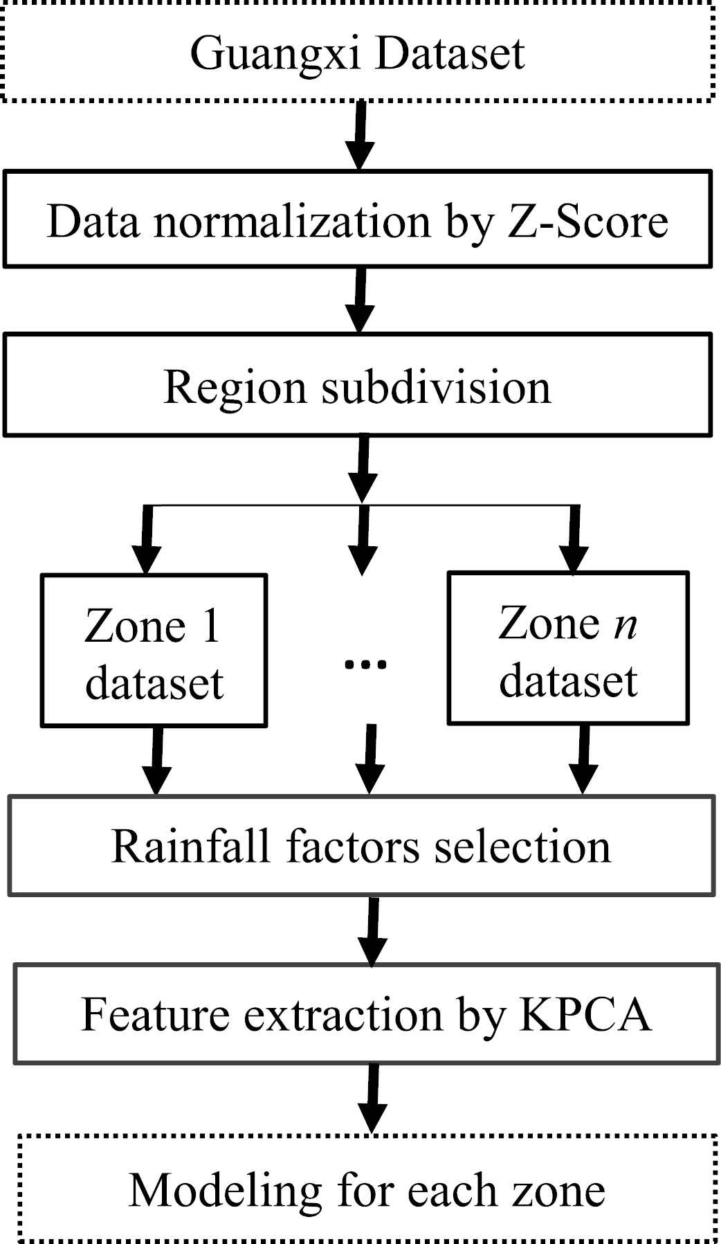
Flowchart of data preprocessing for Guangxi Datasets.
Data Normalization: The Guangxi datasets had been conducted preliminary data cleaning and feature screening by the datasets collectors Guangxi Meteorological Information Center. Therefore, in this work, we firstly conducted data normalization using Z-Score in the data preprocessing of Guangxi Datasets.
Region Subdivision: Different areas of Guangxi are usually characterized by different complex topography, and numerous factors affect precipitation, resulting in the uneven distribution of precipitation. Prediction by dividing sub-regions could not only capture continuous and smooth precipitation patterns within smaller areas to more accurately grasp over the region precipitation patterns but also decrease the complexity of prediction. Therefore, in this work, we separated the predicting area into several sub-regions (i.e. zones) based on the historical precipitation data of Guangxi region, then forecast models are built for each zone. To achieve this, we divided all the 89 stations of Guangxi into three zones with the correlation coefficient larger than 0.35 (significance level of 0.001), as shown in Figure 6.
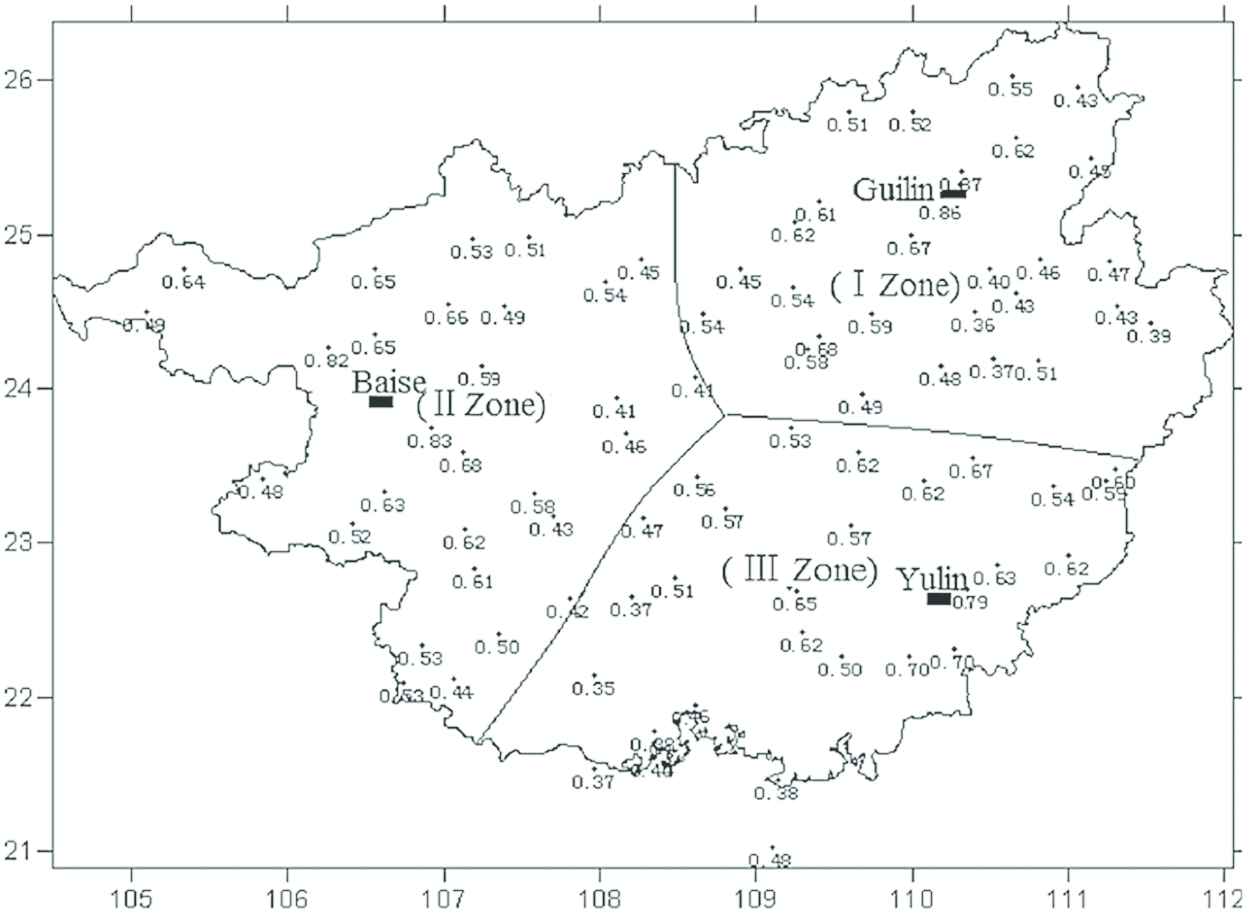
Three zones from the 89 meteorological stations in Guangxi and the correlation coefficient of the stations in each zone relating to the central station of the zone [27]. The correlations of the historical precipitation data in the related region absolutely above 0.37 (99% significance test).
Rainfall Factors Selection: We firstly took the real rainfall sequence and all precipitation grid point sequence of T213 and JMA numerical prediction model in each zone, respectively, with relevant coefficient larger than 0.2 as rainfall field primary factors. Finally, twenty-nine to sixty-eight primary factors of rainfall prediction in different sub-regions were selected.
Feature Extraction: In general, unsuitably selecting a large number of input parameters (dimensions) [39] would lead to over-fitting problem of prediction algorithms. So, We extracted feature from related factors of prediction object area in order to reduce data dimensions and promote prediction performance.
Because precipitation change is a complex nonlinear process, there are strong nonlinear couplings between the primary factors. They increase the difficulty of rainfall prediction. Against this problem, we developed Kernel Principal Component Analysis (KPCA) with Gauss kernel function to extract feature of the important variables affecting rainfall. KPCA is a nonlinear transformation based on the original input data, can extract well the nonlinear relationship between the properties of input meteorological data [22,40].
Comparing with other popular feature extraction methods, we investigated the superior performance of KPCA incorporated with ELM-GEP by taking the zone 3 of the Guang-5 dataset as a case, due to the relatively simple terrain and predictability of the zone 3. In this investigation, we used the forecast result of T213 as the baseline. T213 is the fourth generation of global medium-term NWP system developed by China National Weather Center and widely used in business operation of Chinese meteorological departments. Figure 7 shows the prediction results of ELM-GEP coupled with different popular feature extraction methods. It reveals that KPCA is a very promising feature extraction method in the precipitation prediction in this study.
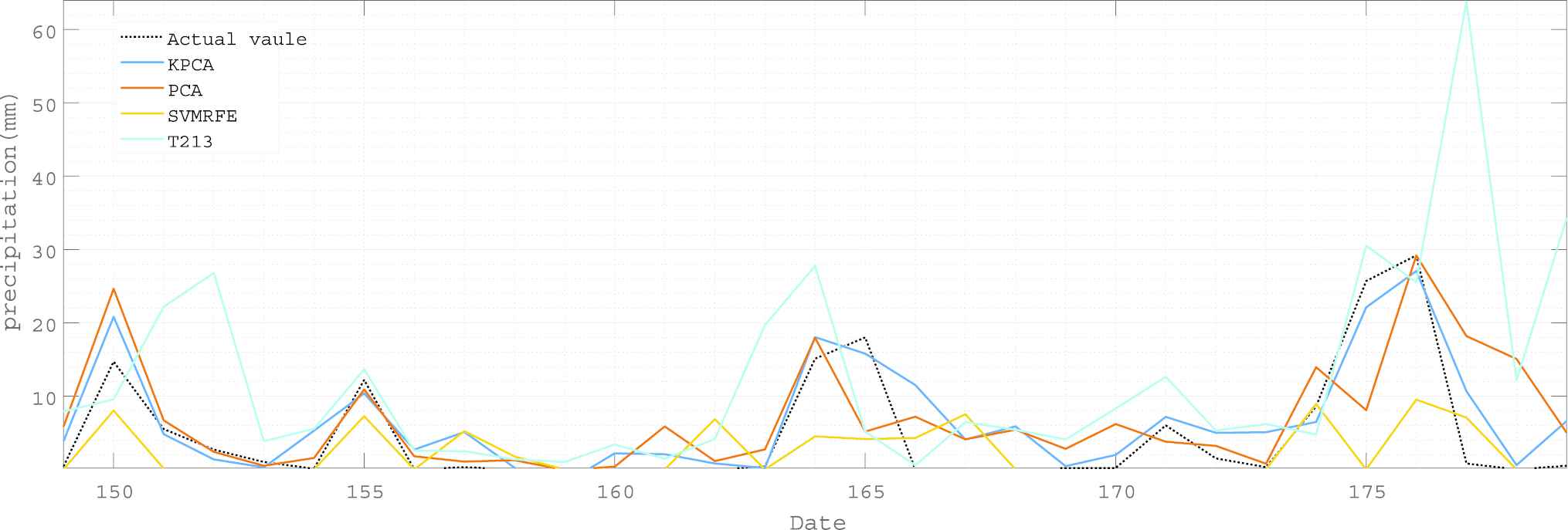
Prediction result of the proposed model with various popular feature extraction methods on zone 3 of Guangxi in May. The cumulative contribution rate was set 90% for both Principal Component Analysis (PCA) and Kernel Principal Component Analysis (KPCA). It was gradually increased the number of selected feature from 1 to 30 for Support Vector Machine Recursive Feature Elimination (SVM-RFE), and then selected the best modeling performance as the final one, which contained the first 28 variables as features.
4.3.3. 48-hours-ahead daily precipitation prediction
In this section, we compare ELM-GEP with the five state-of-the-art models for 48-hours-ahead daily precipitation prediction. For fairness, these models will be subject to the same data-preprocessing process described in Section 4.3.2, except DNN. Here KPCA will not be used in DNN to extract features, as the feature learning in DNN usually performs automatically. We demonstrate the prediction performance of various prediction methods coupled with KPCA or non-coupled in this section. For simplicity, a method likes ELM coupled with KPCA for feature extraction will be abbreviated as “ELM+.”
The comparison results on Guang-4, Guang-5 and Guang-6 datasets are presented in Tables 4–6, respectively. We can see that these methods work with KPCA can always obtain better performance than the ones without KPCA. This means using KPCA to do feature extraction is able to improve the learning ability of these methods in the problem of precipitation prediction.
We can also see that our methods obtained the best MAE and RMSE (the mAve and rAve columns in the Tables 4–6, respectively) in all cases, which means ELM-GEP+ introduces less prediction error than the other methods. We further use t-test to demonstrate that our method can always obtain a better performance than the other methods. The t-test comparison results are presented in the mP-value and rP-value columns in the Tables 4–6. It can be seen that most of the P-values are smaller than the significance level 0.05. This means the proposed method significantly outperforms the five state-of-the-art methods in terms of MAE and RMSE on the Guangxi datasets.
In view of business operation, our proposed model achieves good performances in terms of PRC, SC, ratio and UB Ratio on all Guangxi datasets. All the SC ratios obtained by our proposed model are greater than or equal to 0.533, and most of them are greater than or equal to 0.800. This result reaches a very high level of business operation, while most of SC ratios obtained by T213 model, which developed and used by China Meteorological Administration, in the same period and region are smaller than 0.500. It means that our proposed model has strong fitting ability and generalization ability of precipitation problem.
As a conclusion, our method is able to obtain a better performance than the existing methods on 48-hours-ahead daily precipitation prediction, and the corresponding prediction results are reliable in view of business operation.
4.4. Discussion
The experimental results across all datasets in this work show that: (1) ELM-GEP is a promising soft computing method for regional daily precipitation prediction; (2) By and large, the model based on ELM-GEP wins the best prediction performance across all metrics on all datasets; (3) The features used in model importantly affect the prediction performance. When there are few important variables affecting precipitation prediction, ELM-GEP is also a good model for precipitation prediction without feature extraction, as shown in Section 4.2. When there are many important variables affecting precipitation prediction, ELM-GEP coupled with KPCA (for feature extraction) is significant for precipitation prediction, as shown in Section 4.3.
It should be noted that ELM-GEP is worse than ELM in terms of time complexity. However, we only concentrate on reasonable prediction accuracy and reliability, because the accuracy and the reliability are more important than the time complexity in the daily precipitation prediction.
5. CONCLUSION
This paper presented a novel hybrid model based on ELM and GEP for regional daily quantitative precipitation prediction. Our proposed model can reduce the risk of ELM modeling error using GEP to improve the prediction performance. The proposed model, compared with five state-of-the-art precipitation prediction methods including DNN, ELM, SVR, BP and NARX, was test for solving two different types of daily precipitation prediction problems. The prediction performance was evaluated in terms of five metrics on eight datasets. The comparison results indicate that most of the models can achieve a reasonable prediction accuracy. More importantly, by and large, the proposed model outperforms the state-of-the-art precipitation prediction methods on all datasets with the highest accuracy, and the highest strong credibility and the lowest unreliability.
It would be an interesting topic to research the inclusion of other meteorological elements and materials in future, like air mass trajectories and the satellite cloud picture, which may further improve the forecasting accuracy.
CONFLICT OF INTEREST
There are no conflicts of interest.
AUTHORS' CONTRIBUTIONS
Yuzhong Peng; data curation: Huasheng Zhao, Jie Li and Zhiping Liu; formal analysis: Hao Zhang, Jie Li; methodology: Yuzhong Peng; writing, original draft: Yuzhong Peng, Huasheng Zhao; writing, reviewing and editing: Yuzhong Peng, Huasheng Zhao, Hao Zhang, Jie Li, Wenwei Li, Xiao Qin, Jianping Liao and Zhiping Liu.
ACKNOWLEDGMENTS
We highly appreciate that this work was supported in part by the National Natural Science Foundation of China under Grant #61562008 and #41575051, the Natural Science Foundation of Guangxi Province under Grant #2017GXNSFAA198228 and #2017GXNSFBA198153, the Project of Scientific Research and Technology Development in Guangxi under Grant #AA18118047 and #AD18126015, the basic ability promotion project of young and middle-aged teachers in Guangxi universities #2017KY0896, and the grant of BAGUI Scholar Program of Guangxi Zhuang Autonomous Region of China. Jie Li is the corresponding author.
REFERENCES
Cite this article
TY  - JOUR
AU  - Yuzhong Peng
AU  - Huasheng Zhao
AU  - Hao Zhang
AU  - Wenwei Li
AU  - Xiao Qin
AU  - Jianping Liao
AU  - Zhiping Liu
AU  - Jie Li
PY  - 2019
DA  - 2019/12/04
TI  - An Extreme Learning Machine and Gene Expression Programming-Based Hybrid Model for Daily Precipitation Prediction
JO  - International Journal of Computational Intelligence Systems
SP  - 1512
EP  - 1525
VL  - 12
IS  - 2
SN  - 1875-6883
UR  - https://doi.org/10.2991/ijcis.d.191126.001
DO  - 10.2991/ijcis.d.191126.001
ID  - Peng2019
ER  -