
A New Distance-Based Consensus Reaching Model for Multi-Attribute Group Decision-Making with Linguistic Distribution Assessments
Corresponding author. Email: yaoshengbao@hotmail.com
- DOI
- 10.2991/ijcis.2018.125905656How to use a DOI?
- Keywords
- Multi-attribute group decision-making; Linguistic distribution assessments; Consensus reaching; Distance measure; Optimization
- Abstract
This paper proposes a novel consensus reaching model for multi-attribute group decision making (MAGDM) with information represented by means of linguistic distribution assessments. Firstly, some drawbacks of the existing distance measures for linguistic distribution assessments are analyzed by using numerical counterexamples, and a new distance measure is proposed for linguistic distribution assessments in order to alleviate the limitations. Then, a novel consensus reaching model is developed for MAGDM with linguistic distribution assessment, in which a feedback mechanism is devised by combining an identification rule and an optimization-based model. In this consensus framework, the model allows experts who are identified to modify their preferences to provide additional preference information about linguistic distribution assessments in each iteration. Meanwhile, by solving an optimization model, the consensus reaching model can automatically generate preference adjustment suggestions for experts. Moreover, the optimization model solved in each iteration minimizes the deviation between the adjusted values and initial preferences, which in turn leads to the good performance of the proposed consensus reaching model in preserving the initial preference information. Finally, an illustrative example shows that the proposed consensus reaching model is feasible and effective, and a comparative analysis highlights the advantages and characteristics of the model.
- Copyright
- © 2019 The Authors. Published by Atlantis Press SARL.
- Open Access
- This is an open access article distributed under the CC BY-NC 4.0 license (http://creativecommons.org/licenses/by-nc/4.0/).
1. INTRODUCTION
The increasing complexity of the social and economic environment nowadays makes it more and more impracticable for a single decision maker or expert to consider all the relevant factors of a decision-making problem [1]. For this reason, many companies, organizations, and administrations employ multiple members in complex decision-making processes, which is known as group decision-making (GDM). Generally, GDM can be understood as a process to aggregate individual opinions of multiple experts so as to acquire a group opinion in the situations where experts verbalize their preferences regarding multiple alternatives [2].
Many GDM problems present quantitative aspects which can be evaluated by means of exact numerical values. However, some problems present also qualitative features that are complex to assess by using precise numerical values. In this circumstances, experts usually articulate their preferences with qualitative information that are represented by linguistic variables. In the classical linguistic computational models [3, 4], experts are restricted to express their opinions with a single linguistic term. In complex decision problem under uncertainty, experts may hesitate between different linguistic terms and require richer expressions to express their preferences more accurately. For this reason, Rodríguez et al. [5] proposed the concept of hesitant fuzzy linguistic term set (HFLTS), which is used to enhance the flexibility and richness of linguistic elicitation by experts in hesitant situations under qualitative settings [6]. To provide more flexible and richer linguistic expressions, researchers recently have proposed several distribution-based hesitant fuzzy linguistic information such as linguistic distribution assessments [7], possibility distribution for HFLTS [8], proportional HFLTS [9], probabilistic linguistic term set [10, 11], probability-based interpretation for the linguistic expressions [12]. All these distribution-based hesitant fuzzy linguistic information have successfully served to solve decision-making problems for their specified backgrounds. Among these distribution-based hesitant fuzzy linguistic information types, linguistic distribution assessment has received increasing attention from many scholars [13–15]. Our interest in this paper is focused on GDM problem with information represented by means of linguistic distribution assessments.
In GDM, a group of experts initially may have very different opinions due to the different background, knowledge, and experience of experts. Therefore, it is necessary to develop a consensus reaching process (CRP) to help experts achieve agreement. Traditionally, the ideal consensus can be understood as a full and unanimous agreement of all experts preferences with respect to all the feasible alternatives. This type of consensus is an utopian consensus and it is very difficult to achieve in real-world GDM problems, which has led to the use of a new concept called “soft” consensus level [16]. Under the soft consensus framework, the CRP can be modelled as an iterative group discussion process coordinated by a moderator, who helps the experts to make their preferences closer [17]. To date, the CRP based on the “soft” consensus have attracted wide attentions from researchers in the field of GDM [17–23]. In the process of GDM in complex environment, experts may express their preferences by using preference relations (PRs) with fuzzy linguistic information [18]. Accordingly, a variety of consensus models have been developed for GDM problems in which the preferences are represented by means of PRs with fuzzy linguistic information [7, 17, 18, 24–37]. In some GDM situations, the decision information regarding the alternatives is represented in the form of multi-attribute decision matrix. Similarly, when solving the multi-attribute GDM (MAGDM) problems, the CRP is still necessary to reach an agreement among experts before making a common decision. For MAGDM problems in linguistic information environment, authors have also proposed a number of consensus models. For example, Xu et al. [38] developed an interactive consensus model for MAGDM problems with uncertain linguistic information that is evaluated in different unbalanced linguistic label sets. For MAGDM with multi-granular linguistic term sets, Parreiras et al. [39] introduced a flexible consensus scheme which allows one to rationally aggregate the preferences of a group of experts into a consistent collective preference. Later, Rosello et al. [40] proposed a methodology into MAGDM by using consensus within multi-granular linguistic assessments. In order to solve MAGDM problems under an uncertain linguistic environment, Xu et al. [41] proposed a CRP model to help experts reach a satisfactory consensus. From the perspective of social network analysis, Wu et al. [42] introduced a framework to preference estimation and consensus building for multiple criteria GDM with incomplete linguistic information. Sun et al. [43] proposed a new approach to consensus measurement of MAGDM with linguistic PRs. For 2-tuple linguistic MAGDM with incomplete weight information, Zhang et al. [44] presented a consensus reaching model in which a weight-updating model is employed to derive the weights to eliminate the conflict in the group. For MAGDM under uncertain linguistic environment, Pang et al. [45] developed an interactive consensus model with adaptive experts weights. Recently, Zhang et al. [46] proposed a distance-based consensus measure and presented a minimum adjustment distance consensus rule for MAGDM with HFLTS. By using the relative projection model, Zhang et al. [47] proposed a consensus model for MAGDM with hesitant linguistic information on multi-granular linguistic term sets.
Through the above analysis of the relevant literatures, we can see that previous studies have made significant contributions to the consensus models of GDM problems with fuzzy linguistic information. However, a more detailed survey of the literature showed that consensus modeling of MADGM problem with linguistic distribution assessment has not been adequately considered. Therefore, this paper focuses on GDM problems in which the experts express their preferences by means of multi-attribute decision matrix with linguistic distribution assessments. Comparing with the existing consensus models for MAGDM problems, our contributions can be mainly summarized in the following aspects:
As we know, distance and similarity measures play an important role in developing effective CRP model. To study the applications of linguistic distribution assessments, several distance measures between linguistic distribution assessment have been proposed [7, 14, 15]. However, as discussed in Section 3, the existing distance measures are not free from drawbacks. In order to overcome the limitations of the existing distance measures, we propose a novel distance measure for linguistic distribution assessments based on the concept of cumulative proportion distribution. We also find that the proposed distance measure satisfies several desirable properties.
Popular consensus models for MAGDM problems can be divided into the interactive ones and the automatic ones [45]. Generally, the interactive consensus models are usually lack of effective feedback mechanisms to guide the experts to make quick adjustments, while the automatic ones cannot reflect the subjective adjustment opinions from the experts during the CRP. For MAGDM problem with linguistic distribution assessment, a novel consensus reaching model is developed in this paper. The proposed consensus reaching model not only can reflect experts additional preferences during the CRP but also can automatically generate advices for preference adjustment.
One of the most significant issues in the consensus reaching model is how to design an effective feedback mechanism to guide experts reach consensus with minimum adjustments. A hybrid feedback mechanism is designed by combining an identification rule (IR) and an optimization based model in the proposed consensus reaching model. During CRP, an optimization model is solved in each iteration to minimize the the deviation between the adjusted values and initial preferences, which in turn leads to the good performance of the proposed consensus reaching model in preserving the initial preference information.
The rest of the paper is organized as follows: Section 2 summaries the basic concepts of the 2-tuple linguistic representation model and linguistic distribution assessment. In Section 3, we analyze the existing distance measures, and point out their drawbacks with numerical counterexamples. In addition, a novel distance measure is defined for linguistic distribution assessments. Section 4 establishes a consensus support model for MAGDM problems under linguistic distribution assessment environment. Numerical examples and a comparison study are presented in Section 5 to illustrate the performance of the proposed method. Finally, we conclude the paper in Section 6.
2. PRELIMINARIES
This section reviews some relevant knowledge regarding the 2-tuple linguistic representation model and the concept of linguistic distribution assessments.
2.1. Linguistic Information and 2-Tuple Linguistic Representation Model
Suppose that S = {s0, s1, …, sg−1} is a linguistic term set with odd cardinality g, such as 5 or 7, where each label si represents a possible value of a linguistic variable. Usually, it requires that the linguistic term set S satisfies the following characteristics: 1) the set of the linguistic terms is ordered: si ≥ sj if i ≥ j; 2) there exists a negation operator “Neg” such that Neg (si) = sg−i; 3) the maximization operator “max”: max (si, sj) = si if si ≥ sj; and 4) the minimization operator “min”: min (si, sj) = si if si ≤ sj.
In order to avoid information loss in computing with words, Herrera and Martínez [4] introduced the 2-tuple linguistic representation model on the basis of the symbolic translation. In this model, a 2-tuple (si, αi) is used to represent linguistic information, where si is a linguistic term pertaining to the predefined linguistic term set and αi ∈ [−0.5, 0.5) represents the symbolic translation. Specifically, the 2-tuple linguistic representation model is formally defined as follows:
Definition 2.1.
([4]). Let S = {s0, s1, …, sg} be a linguistic term set and β ∈ [0, g] be a value representing the result of a symbolic aggregation operation, then the 2-tuple that expresses the equivalent information to β is obtained with the following function:
According the above definition, a linguistic term si belonging to the linguistic term set S can be regarded as a 2-tuple linguistic by adding a value 0 to it as symbolic translation. That is, si ∈ S ⇒ (si, 0). For convenience’s sake, we will use 2-tuple linguistic representations instead of linguistic terms in the following.
Definition 2.2.
([4]). Let S = {s0, s1, …, sg} be a linguistic term set and (si, αi) be a 2-tuple, there exists a function
Definition 2.3.
([4]). Let x = {(s1, α1), (s2, α2), …, (sn, αn)} be a set of 2-tuples and W = {w1, …, wn} be their associated weights. The 2-tuple weighted average
2.2. Linguistic Distribution Assessments
In [7], Zhang et al. defined the concept of distribution assessments in a linguistic term set. In this subsection, we review some related knowledge regarding linguistic distribution assessment.
Definition 2.4.
[7] Let S = {s0, s1, …, sg−1} be a linguistic term set. Let m = {(sk, βk) | k = 0, 1, …, g − 1}, where
Definition 2.5.
[7] Let m = {(sk, βk) | k = 0, 1, …, g − 1}, where
Zhang et al. [7] developed the following computational model for the distribution assessment of S. Let m1 and m2 be two distribution assessments of S. Then
A comparison operator:
if E (m1) < E (m2), then m1 is smaller than m2;
if E (m1) = E (m2), then m1 and m2 have the same expectation.
A weighted averaging operator of linguistic distribution assessments are defined as follows:
Definition 2.6.
[7] Let {m1, m2, …, mn} be a set of linguistic distribution assessments of S, where
3. AN IMPROVED DISTANCE MEASURE FOR LINGUISTIC DISTRIBUTION ASSESSMENTS
Distance and similarity measures are common tools used widely in measuring the deviation and proximity degrees of different arguments [48]. To study the applications of linguistic distribution assessments, several distance measures between linguistic distribution assessments have been proposed. In this section, we point out some drawbacks of the existing distance measures by counterexamples. Furthermore, we introduce a new distance and similarity measure between linguistic distribution assessments to overcome such drawbacks.
Zhang et al. [7] defined the distance between linguistic distribution assessments m1 and m2 as follows:
Definition 3.1.
[7]: Let
The drawback of the distance measure defined by Eq. (4) is shown with Example 1.
Example 1.
Let Sexample = {s0, s1, s2, s3, s4, s5, s6} be a linguistic term set and there are three linguistic distribution assessments: m1 = {(s0, 0.5), (s1, 0.5), (s2, 0), (s3, 0), (s4, 0), (s5, 0), (s6, 0)}, m2 = {(s0, 0), (s1, 0), (s2, 0), (s3, 0.5), (s4, 0.5), (s5, 0), (s6, 0)}, m3 = {(s0, 0), (s1, 0), (s2, 0), (s3, 0), (s4, 0), (s5, 0.5), (s6, 0.5)}. By Definition 3.1, we can obtain
Zhang et al. [14] pointed out that the distance measure defined by Eq. (4) just calculates the deviation between symbolic proportions and ignores the linguistic terms. To overcome the drawback, Zhang et al. [14] proposed a new distance measure as follows:
Definition 3.2.
[14]: Let
Reconsider Example 1. By Definition 3.2, we can obtain d (m1, m2) = 0.50 and d (m1, m3) = 0.83. Indeed, the distance measure defined by Eq. (5) overcomes the limitation of the distance measure defined by Eq. (4) to a certain extent. However, the distance measure defined by Eq. (5) also has limitation, which can be illustrated by the following Example 2:
Example 2.
Let Sexample = {s0, s1, s2, s3, s4, s5, s6} be a linguistic term set and there are three linguistic distribution assessments: m1 = {(s0, 0), (s1, 0), (s2, 0.1), (s3, 0.8), (s4, 0.1), (s5, 0), (s6, 0)}, m2 = {(s0, 0), (s1, 0.1), (s2, 0.2), (s3, 0.4), (s4, 0.2), (s5, 0.1), (s6, 0)}. Obviously, we can see that m1 and m2 are two different linguistic distribution assessments, that is, m1 ≠ m2. However, by definition 3.2, we obtain d (m1, m2) = 0. According to definition 3.2, it is not difficult to infer that d (m1, m2) = 0 if E (m1) = E(m2). We argue that an ideal distance measure for linguistic distribution assessment should possess the basic property: d (m1, m2) = 0 if and only if m1 = m2.
Recently, Yu et al. [15] defined a new distance measure between linguistic distribution assessments as follows:
Definition 3.3.
[15]: Let
The advantage of the distance measure defined by Eq. (6) can measure the distance between some unequal linguistic distribution assessments which previous distance measurement cannot measure [15]. However, it is not free from drawbacks.
Example 3.
Let Sexample = {s0, s1, s2, s3, s4, s5, s6} be a linguistic term set and there are three linguistic distribution assessments: m1 = {(s0, 0), (s1, 0), (s2, 0)), (s3, 0), (s4, 0), (s5, 0.2), (s6, 0.8)}, m2 = {(s0, 0), (s1, 0), (s2, 0.5), (s3, 0.5), (s4, 0), (s5, 0), (s6, 0)}, m3 = {(s0, 0), (s1, 0), (s2, 0), (s3, 0.5), (s4, 0.5), (s5, 0), (s6, 0)}. By definition 3.3 (r = 1), we can obtain
Based on the above analysis, this paper attempts to develop a new distance measure between distribution assessments by making full use of the proportion distribution information of linguistic distribution assessment. Similar to the cumulative probability distribution, the concept of cumulative proportion distribution can be derived for linguistic distribution assessment. In particular, the vector
Definition 3.4.
Let
Example 4.
Reconsider the linguistic distribution assessments in Example 2: m1 = {(s0, 0), (s1, 0), (s2, 0.1), (s3, 0.8), (s4, 0.1), (s5, 0), (s6, 0)}, m2 = {(s0, 0), (s1, 0.1), (s2, 0.2), (s3, 0.4), (s4, 0.2), (s5, 0.1), (s6, 0)}. For m1 and m2, we can calculate their cumulative proportion distributions CP1 = (0, 0, 0.1, 0.9, 1, 1, 1) and CP2 = (0, 0.1, 0.3, 0.7, 0.9, 1, 1). By using Eq. (7), we have d (m1, m2) = 0.1. It is worth noting that the proposed distance measure defined by Eq. (7) has very clear geometric meaning. Figure 1 shows the proportion distribution of linguistic distribution assessments m1 and m2 (for convenience, the subscripts of linguistic term are taken as the values of variable). The distance d (m1, m2) between two linguistic distribution assessments m1 and m2 can be explained as the ratio of intersecting area of the corresponding cumulative proportion distributions and g − 1. From Figure 1, we can see that the distance d (m1, m2) equals the ratio of the sum of area of S1, S2, S3, S4, and the area of rectangle OABC. Clearly, the larger the intersecting area between the two cumulative proportion distributions is, the farther the distance between the two linguistic distribution assessments is.
The geometric interpretation of the proposed distance measure.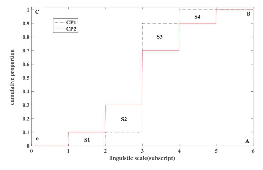
In order to analyze the performance of the proposed distance measure, we conduct a comparative analysis by using numerical examples. Reconsider Example 1, Example 2, and Example 3. We calculate the values of the distance by applying the proposed distance measure defined by Equation (7) and the existing distance measures defined by Equations. (4–6). Table 1 shows the comparison results. As we can see from Table 1 on the one hand, the existing distance measures show some limitations, which has been explained in detail in section 3. On the other hand, we can also see that the proposed distance measure in this paper not only can distinguish linguistic distribution assessments as shown in Example 1, in which the positive proportions are distributed on different linguistic terms, but also can distinguish linguistic distribution assessments with the same expectation values. Moreover, for the linguistic distribution assessments in Example 3, the results calculated by the proposed distance measure are more reasonable than that calculated by the distance measure proposed in [15]. From above analysis, we can conclude that the proposed distance measure for linguistic distribution assessments exhibits better performance.
| Equation (4) Zhang et al. [7] | Equation (5) Zhang et al. [14] | Equation (6) Yu et al. [15] | Equation (7) The Proposed Measure | |
|---|---|---|---|---|
| Example 1 | d (m1, m2) = 1, d (m1, m3) = 1 | d (m1, m2) = 0.50, d (m1, m3) = 0.83 | d (m1, m2) = 0.21, d (m1, m3) = 0.38 | d (m1, m2) = 0.50, d (m1, m3) = 0.83 |
| Example 2 | d (m1, m2) = 0.4 | d (m1, m2) = 0 | d (m1, m2) = 0.06 | d (m1, m2) = 0.10 |
| Example 3 | d (m1, m2) = 1, d (m1, m3) = 1 | d (m1, m2) = 0.55, d (m1, m3) = 0.38 | d (m1, m2) = 0.16, d (m1, m3) = 0.20 | d (m1, m2) = 0.55, d (m1, m3) = 0.38 |
Calculation results of different distance measure for linguistic distribution assessments.
For the proposed distance measure, we can obtain the following properties.
Theorem 3.1.
Let
Then the distance measure defined by Eq. (7) satisfies the following properties:
d (m1, m2) ≥ 0;
d (m1, m2) = d (m2, m1);
d (m1, m2) = 0 if and only if m1 = m2, i.e.,
d (m1, m2) = 1 if and only if m1 = mmin (or mmax), m2 = mmax (or mmin)
where mmin = {(s0, 1), …, (sg − 1, 0)} and mmax = {(s0, 0), …, (sg − 1, 1)};
d (m1, m2) ≤ d (m1, m3) + d (m3, m2).
Proof.
(1) and (2) are obvious.
(3). According to Definition 3.4, d (m1, m2) = 0 holds if and only if
(4) Notice that
This completes the proof of Theorem 3.1.
Definition 3.5.
Let
Obviously, 0 ≤ s (m1, m2) ≤ 1. The closer s (m1, m2) is to 1, the more similar m1 is to m2, while the closer s (m1, m2) is to 0, the more distant m1 is from m2.
4. A CONSENSUS SUPPORT MODEL FOR MAGDM WITH LINGUISTIC DISTRIBUTION ASSESSMENTS
In this subsection, we describe the framework of the proposed consensus reaching model for MAGDM with linguistic distribution assessments.
4.1. The Framework of the Proposed Consensus Support Model
Consider a MAGDM problem with linguistic distribution assessments. Let X = {x1, x2, …, xm} be a discrete set of m (m ≥ 2) potential alternatives, C = {c1, c2, …, cn} be the set of n (n ≥ 2) attributes or criteria. Suppose that W = {w1, w2, …, wn}T is the weight vector of attributes, such that
Remark 1.
In the considered MAGDM problem, it is assumed that preferences of experts are represented by using linguistic distribution assessments. Although linguistic distribution assessment can be used to enhance the flexibility and richness of linguistic elicitation by experts in hesitant situations under qualitative settings, experts may have some cognitive difficulties in using linguistic distribution assessments to articulate their preferences in practice. Especially, experts may find it difficult to provide proportional distribution information on HFLTS with too many linguistic terms. Therefore, in practice, it is suggested that experts should provide the proportional distribution information on HFLTS with no more than three linguistic terms when articulating preferences by using linguistic distribution assessments.
A typical resolution method for a GDM problem consists of two different processes: the consensus process and the selection process. The consensus process refers to how to obtain the maximum degree of consensus or agreement among the experts on the solution alternatives, while the selection process consists in how to obtain the solution set of alternatives from the opinions on the alternatives given by the experts. Inspired by these two processes, we propose the framework of the MAGDM with linguistic distribution assessments. The details of the framework are described in Figure 2. As we know, the feedback mechanism is the core part of a consensus reaching model. There are three main steps in the proposed feedback mechanism. In the first step, an IR is implemented to locate the experts who need to reevaluate his/her assessment values and the position where he/she need to modify. In the second step, an optimization model is established to minimize the deviation between the adjusted values and initial preferences. Simultaneously, additional preference information provided by the experts is also incorporated into the optimization model. By solving the constructed optimization model, adjustment advices are generated in the third step. The details of the consensus process are introduced in the following subsections.
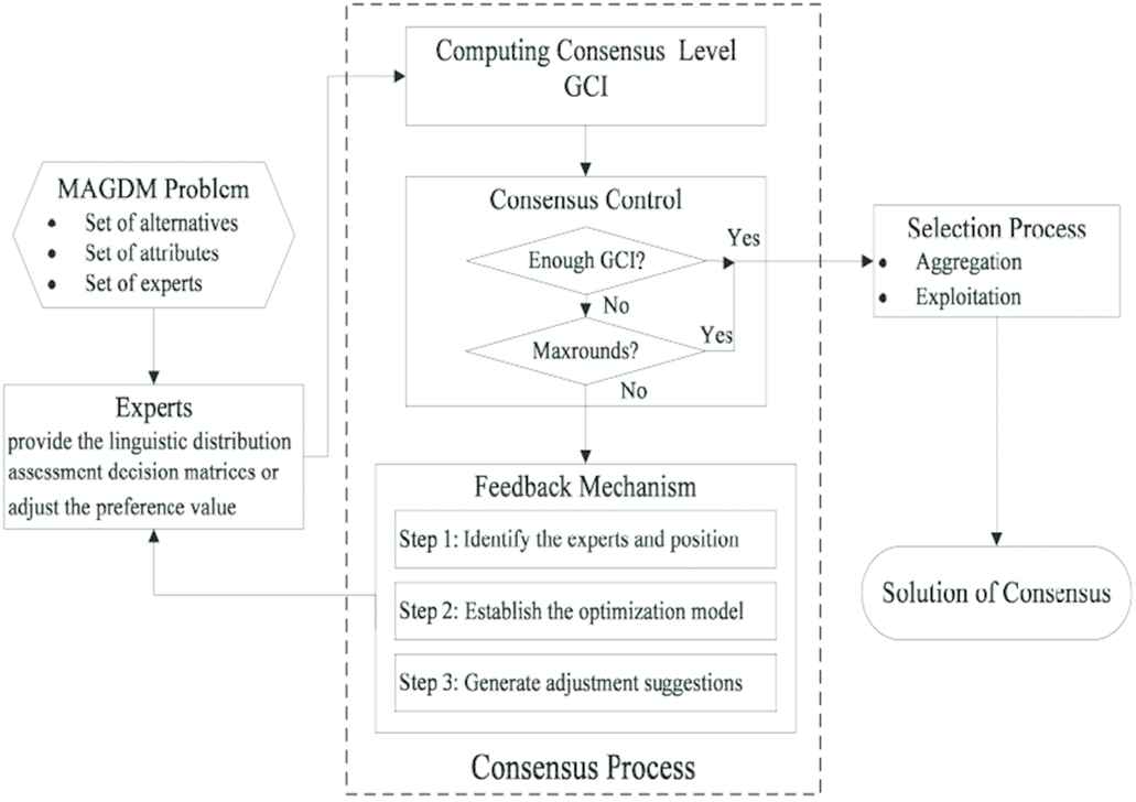
The resolution framework for multi-attribute group decision- making (MAGDM) problem with LDA.
4.2. The Consensus Measure
The weighted averaging operator DAWAλ can be used to transform individual linguistic distribution assessment decision matrix Mt = (mij,t)m×n, t ∈ {1, 2, …, T} into the following collective decision matrix Mcol = (mij,col)m×n:
Based on the similarity degree of two linguistic distribution assessments, for each expert et (t = 1, 2, …, T), a similarity matrix
There are T similarity matrices. By aggregating all the similarity matrices St,col (t = 1, 2, …, T) associated with each expert et, we can obtain a consensus matrix
The aggregation is conducted using an weighted aggregation operator Agg,
In the following, based on the consensus matrix, the group consensus index can be defined.
Definition 4.1.
The group consensus index GCI for the decision matrices Mt (t = 1, 2, …, T) is defined as
The group consensus index GCI is defined to measure the overall consensus level among the decision makers’ decision matrices and is used to control the process of the consensus reaching. Although the group consensus level GCI can be calculated using the arithmetic mean of all the consensus degrees on the attribute values, here we adopt a min operator to allow for a more rigorous criterion. In this way, a compromise is avoided between some attribute values with very high consensus degrees and those with very low consensus degrees.
Obviously, 0 ≤ GCI ≤ 1. The larger the value of GCI, the closer that the experts are to each others. The threshold of consensus level
4.3. The Feedback Mechanism
When comparing the current consensus level GCI with the predefined consensus threshold value
(a) Identification rules: The IRs are utilized to identify attribute values provided by the experts that are contributing less to the attainment of a high consensus level. In the CRP for MAGDM, the IR are given to locate which expert need to reevaluate his/her assessment values and in which specific position he/she need to modify. Here, we define the set IDE that contains 3-tuples (t, i, j) symbolizing attribute values mij,t that should be changed because they affect badly to that consensus state. To compute IDE, we apply a two step identification process that uses the consensus measures previously defined.
Identification of position (i, j):
Identification of expert-position (t, i, j):
(b) Recommendation rules: The RRs are to generate personalized advices to help experts to change their evaluation matrices. For each (t, i, j) ∈ IDE, the RRs will give recommendations for adjusting the corresponding attribute value. The RRs of the proposed model is based on an optimization model. At each iteration of our method, an optimization model is established for each (i, j) ∈ POS. By solving the optimization model, suggestions will be generated for all experts who need to adjust preferences in the position (i, j). The model proposed in this paper has two prominent characteristics. Firstly, the adjustment of attribute values takes into account the additional preference information from the experts. Secondly, under the condition that the group consensus level is improved, the optimization model protects the expert initial preference information by minimizing the adjustments.
Let
Δij determined by the Equation (17) can guarantee that after the adjustment of preference values, the group consensus level in the position (i, j) can either reach the threshold
In order to reflect the real preferences of decision makers, the proposed consensus reaching model allows decision makers to provide additional preference information at each iteration. It is supposed in our model that decision makers are willing to provide preference information about deviations
Clearly, the variables
In model (M − 3), the objective is to minimize the weighted sum of all deviation variables for
4.4. An Iterative Algorithm for CRP
For a MAGDM problem, let Mt = (mij,t) m×n be the decision matrix given by the expert et ∈ E, where
Algorithm 1. (Consensus reaching process)
Input: Mt = (mij,t)) m×n, et ∈ E, the maximum number of iterative times Roundmax, the threshold of group consensus level
Output: Improved decision matrices
Step 1. Initiate the procedure. Let l = 0 and
Step 2. Utilize the operator DAWAλ to fuse all individual decision matrices
Step 3. Calculate the similarity matrix
Step 4. Aggregate all the similarity matrices
Step 5. Determine the group consensus index GCI(l) by using (15). if
Step 6. Identify attribute values
Locate the position (i, j) by using (16), that is,
and determine the set
Let IDE(l) be the set that contains 3-tuples (t, i, j) symbolizing attribute values
Step 7. Elicit preference information about
Step 8. Solve the optimization model (M − 3). Denote the optimal solution of model (M − 3) as
Step 9. Adjust the linguistic distribution assessments
Step 10. Determine the updated consensus matrix
Step 11. Output
Step 12. End.
The proposed Algorithm 1 is an iterative process which can improve the group consensus level. Regarding convergence of Algorithm 1, we can prove the following Theorem 4.1.
Theorem 4.1.
Let Mt = (mij,t) m×n be the T individual decision matrices, let
Proof.
According to Definition 4.1 and Algorithm 1, we have
Therefore, if
Theorem 4.1 shows that the group consensus level GCI(l) is increasing in the process of iteration. Since the parameter ε is positive, we can always obtain an improved decision matrix for each expert, which satisfies the predefined consensus level
Remark 2.
From Algorithm 1, we can see that although additional preferences of experts are considered in the proposed CRP, experts don’t need to provide preferences in the form of linguistic distribution assessments during iteration of CRP. In fact, experts only need to provide preferences about the adjustment range of the proportional distribution information on HFLTS.
4.5. The Selection Process
Once the group consensus level amongst experts has been achieved, we can obtain a group decision matrix
Based on the updated collective decision matrix
5. NUMERICAL ANALYSIS
5.1. Numerical Example
In this section, an example of investment decision problem is used to illustrate the practicality and effectiveness of the proposed consensus-based decision- making model. In this example, an investment company wants to invest a sum of money in the best industrial sector. Suppose that there are four possible alternatives A = {A1, A2, A3, A4}, where A1 is the car industry, A2 is the food industry, A3 is the computer industry, and A4 is the weapons industry. To best serve the interests of shareholders, three experts E = {e1, e2, e3 from three departments within the company are invited to offer suggestions: e1 is from the risk analysis department, e2 from the growth analysis department, e3 from the environmental impact analysis department. Equal weights are assumed for the three experts. Each expert was asked to provide their assessments over the four candidates with respect to the following four attributes: C1-the ability of sale, C2-the ability of production, C3-the ability of technology, C4-the ability of financing. The weight vector of attributes is W = (0.25, 0.25, 0.25, 0.25). Suppose that the experts evaluate the performance of each alternative by using linguistic distribution assessments. The linguistic term set used by the experts is S = {s0 = extremely poor, s1 = very poor, s2 = poor, s3 = fair, s4 = good, s5 = very good, s6 = extremely good}. Individual decision matrices for each expert are listed in Tables 2–4. In this example, the following set of parameters is used:
| mij,1 | C1 | C2 | C3 | C4 |
|---|---|---|---|---|
| A1 | m11,1 = {(s2, 0.2), (s3, 0.5), (s4, 0.3)} | m12,1 = {(s4, 0.2), (s5, 0.6), (s6, 0.2)} | m13,1 = {(s3, 0.3), (s4, 0.4), (s5, 0.3)} | m14,1 = {(s3, 0.2), (s4, 0.6), (s5, 0.2)} |
| A2 | m21,1 = {(s3, 0.6), (s4, 0.2), (s5, 0.2)} | m22,1 = {(s4, 0.7), (s5, 0.3)} | m23,1 = {(s2, 0.4), (s3, 0.5), (s4, 0.1)} | m24,1 = {(s5, 0.7), (s6, 0.3)} |
| A3 | m31,1 = {(s4, 0.3), (s5, 0.7)} | m32,1 = {(s1, 0.3), (s2, 0.6), (s3, 0.1)} | m33,1 = {(s2, 0.5), (s3, 0.4), (s4, 0.1)} | m34,1 = {(s5, 0.6), (s6, 0.4)} |
| A4 | m41,1 = {(s2, 0.2), (s3, 0.4), (s4, 0.4)} | m42,1 = {(s4, 0.6), (s3, 0.4), (s5, 0.2)} | m43,1 = {(s3, 0.4), (s4, 0.4), (s5, 0.2)} | m44,1 = {(s4, 0.3), (s5, 0.7)} |
The individual linguistic distribution assessments matrix M1.
| mij,2 | C1 | C2 | C3 | C4 |
|---|---|---|---|---|
| A1 | m11,2 = {(s2, 0.3), (s3, 0.3), (s4, 0.4)} | m12,2 = {(s4, 0.4), (s5, 0.6)} | m13,2 = {(s3, 0.3), (s4, 0.3), (s5, 0.4)} | m14,2 = {(s2, 0.5), (s3, 0.3), (s4, 0.2)} |
| A2 | m21,2 = {(s2, 0.1), (s3, 0.4), (s4, 0.5)} | m22,2 = {(s3, 0.5), (s4, 0.2), (s5, 0.3)} | m23,2 = {(s3, 0.3), (s4, 0.5), (s5, 0.2)} | m24,2 = {(s5, 0.4), (s6, 0.6)} |
| A3 | m31,2 = {(s4, 0.4), (s5, 0.6)} | m32,2 = {(s1, 0.2), (s2, 0.2), (s3, 0.6)} | m33,2 = {(s2, 0.3), (s3, 0.4), (s4, 0.3)} | m34,2 = {(s4, 0.2), (s5, 0.6), (s6, 0.2)} |
| A4 | m41,2 = {(s2, 0.5), (s3, 0.4), (s4, 0.1)} | m42,2 = {(s3, 0.3), (s4, 0.5), (s5, 0.2)} | m43,2 = {(s4, 0.1), (s5, 0.2), (s6, 0.7)} | m44,2 = {(s4, 0.3), (s5, 0.5), (s6, 0.2)} |
The individual linguistic distribution assessments matrix M2.
| mij,3 | C1 | C2 | C3 | C4 |
|---|---|---|---|---|
| A1 | m11,3 = {(s3, 0.7), (s4, 0.3)} | m12,3 = {(s5, 0.8), (s6, 0.2)} | m13,3 = {(s3, 0.2), (s4, 0.6), (s5, 0.2)} | m14,3 = {(s3, 0.1), (s4, 0.5), (s5, 0.4)} |
| A2 | m21,3 = {(s2, 0.2), (s3, 0.6), (s4, 0.2)} | m22,3 = {(s4, 0.6), (s5, 0.4)} | m23,3 = {(s2, 0.5), (s3, 0.3), (s4, 0.2)} | m24,3 = {(s5, 0.4), (s6, 0.6)} |
| A3 | m31,3 = {(s2, 0.3), (s3, 0.3), (s4, 0.4)} | m32,3 = {(s1, 0.1), (s2, 0.7), (s3, 0.2)} | m33,3 = {(s2, 0.2), (s3, 0.3), (s4, 0.5)} | m34,3 = {(s4, 0.2), (s5, 0.6), (s6, 0.2)} |
| A4 | m41,3 = {(s2, 0.4), (s3, 0.2), (s4, 0.4)} | m42,3 = {(s3, 0.2), (s4, 0.6), (s5, 0.2)} | m43,3 = {(s3, 0.4), (s4, 0.3), (s5, 0.3)} | m44,3 = {(s5, 0.7), (s6, 0.3)} |
The individual linguistic distribution assessments matrix M3.
Firstly, we use Algorithm 1 (CRP) to help experts achieve a consensus.
Step 1. Initiate the procedure. Let l = 0, and
Step 2. Calculate the collective decision matrix. By using the operator DAWAλ, the collective decision matrix is obtained and shown in Table 5.
| mij,col | C1 | C2 | C3 | C4 |
|---|---|---|---|---|
| A1 | m11,col = {(s2, 0.17), (s3, 0.50), (s4, 0.33)} | m12,col = {(s4, 0.20), (s5, 0.67), (s6, 0.13)} | m13,col = {(s3, 0.27), (s4, 0.43), (s5, 0.30)} | m14,col = {(s2, 0.17), (s3, 0.20), (s4, 0.43), (s5, 0.20)} |
| A2 | m21,col = {(s2, 0.10), (s3, 0.53), (s4, 0.30), (s5, 0.07)} | m22,col = {(s3, 0.17), (s4, 0.50), (s5, 0.33)} | m23,col = {(s2, 0.30), (s3, 0.37), (s4, 0.27), (s5, 0.06)} | m24,col = {(s5, 0.50), (s6, 0.50)} |
| A3 | m31,col = {(s2, 0.10), (s3, 0.10), (s4, 0.37), (s5, 0.43)} | m32,col = {(s1, 0.20), (s2, 0.50), (s3, 0.30)} | m33,col = {(s2, 0.33), (s3, 0.37), (s4, 0.30)} | m34,col = {(s4, 0.13), (s5, 0.60), (s6, 0.27)} |
| A4 | m41,col = {(s2, 0.37), (s3, 0.33), (s4, 0.30)} | m42,col = {(s3, 0.17), (s4, 0.57), (s5, 0.20), (s6, 0.06)} | m43,col = {(s3, 0.30), (s4, 0.30), (s5, 0.40)} | m44,col = {(s4, 0.20), (s5, 0.63), (s6, 0.17)} |
The collective decision matrix
Step 3. By using the similarity measure, we can obtain the similarity matrices between each individual decision matrix and the collective decision matrix. In the first round, we obtain the the similarity matrices
Step 4. By using Eq. (14), the similarity matrices can be aggregated into the consensus matrix
Step 5. Based on the consensus matrix
Step 6. By using the IRs, we can locate the experts need to reevaluate his/her assessment values and specific position in which he/she need to modify. We obtain IDE(0) = {(1, 3, 1), (3, 3, 1)}, which means that experts e1 and e3 should modify their preferences about alternative A3 with respect to attribute C1.
Step 7. Elicit preference information about
Suppose that experts e1 and e3 provide the following additional preferences:
Step 8. Based on the preference information provided by experts e1 and e3, the optimization model (M − 3) can be constructed. By solving the optimization model, we obtain the following nonzero components of the optimal solution:
Step 9. Adjust the linguistic distribution assessments. According to the optimal solution of the model (M − 3), we can see that only the expert e3 need to adjust his preference in position (3, 1). The adjusted preference is
Step 10. Determine the updated consensus matrix. Based on the modified decision matrices, we can calculate the updated consensus matrix
We can see that
In this example, the predefined consensus level is achieved after six rounds of iterations. Compared with the original decision matrices, the expert e1 does not adjust his preferences. The expert e2 updates the preference m14,2 and m23,2 to
| xij | C1 | C2 | C3 | C4 |
|---|---|---|---|---|
| A1 | m11,col = {(s2, 0.17), (s3, 0.50), (s4, 0.33)} | m12,col = {(s4, 0.20), (s5, 0.67), (s6, 0.13)} | m13,col = {(s3, 0.27), (s4, 0.43), (s5, 0.30)} | m14,col = {(s2, 0.14), (s3, 0.16), (s4, 0.45), (s5, 0.25)} |
| A2 | m21,col = {(s2, 0.10), (s3, 0.53), (s4, 0.30), (s5, 0.07)} | m22,col = {(s3, 0.20), (s4, 0.60), (s5, 0.20)} | m23,col = {(s2, 0.31), (s3, 0.37), (s3, 0.27), (s5, 0.05)} | m24,col = {(s5, 0.50), (s6, 0.50)} |
| A3 | m31,col = {(s2, 0.08), (s3, 0.05), (s4, 0.37), (s5, 0.50)} | m32,col = {(s1, 0.20), (s2, 0.05), (s3, 0.30)} | m33,col = {(s2, 0.33), (s3, 0.37), (s4, 0.30)} | m34,col = {(s4, 0.13), (s5, 0.60), (s6, 0.27)} |
| A4 | m41,col = {(s2, 0.33), (s3, 0.33), (s4, 0.34)} | m42,col = {(s3, 0.17), (s4, 0.57), (s5, 0.20), (s6, 0.06)} | m43,col = {(s3, 0.23), (s4, 0.37), (s5, 0.33), (s6, 0.07)} | m44,col = {(s4, 0.20), (s5, 0.63), (s6, 0.17)} |
The final collective decision matrix Mcol.
In the following, the selection process of the GDM model is implemented.
Based on the final collective decision matrix Mcol, we can obtain the following overall values of each alternative by using the known weights of attributes and DAWAW operator: m1,col = {(s2, 0.08), (s3, 0.25), (s4, 0.35), (s5, 0.29), (s6, 0.03), m2,col = {(s2, 0.11), (s3, 0.29), (s4, 0.28), (s5, 0.22), (s6, 0.10), m3,col = {(s1, 0.05), (s2, 0.23), (s3, 0.18), (s4, 0.21), (s5, 0.27), (s6, 0.06), m4,col = {(s2, 0.11), (s3, 0.22), (s4, 0.35), (s5, 0.28), (s6, 0.04),
By using Eq. (2), we can further obtain the expectation of each alternative, i.e., E(m1,col) = (s4, –0.0455), E(m2,col) = (s4, –0.0933), E(m3,col) = (s4, –0.4197), E(m4,col) = (s4, –0.0600). According to the values of E(mi,col), i = 1, 2, 3, 4, the ranking of four alternatives is x1 ≻ x4 ≻ x2 ≻ x3.
5.2. Comparison Analysis
In order to demonstrate the differences between the proposed method and other relevant methods and emphasize the advantages and characteristics of the proposed method, in this section we conduct comparison analysis to evaluate the performance of the proposed consensus reaching model.
Regarding MAGDM problem with linguistic distribution assessments, a consensus reaching model is proposed in this paper to help decision makers to achieve agreement in decision-making. In order to analyze the impact of CRP on decision-making, by using the numerical example in Section 5, we compare the result calculated by our model with that calculated by the MAGDM model without CRP. In the numerical example, we can aggregate the original individual decision matrices by using the DAWAW operator. Further, based on the collective decision matrix, that is,
In [7], Zhang et al. developed a consensus model for GDM with linguistic distribution assessments based on the IR and the adjustment rule. Here, we compare the consensus model in [7] and the proposed consensus model in the present paper from the following aspects. In the first place, although both models are concerned with consensus issue in GDM problems with linguistic distribution assessments, the proposed consensus model is developed for GDM problems in which the decision information is represented by means of multi-attribute decision matrix, while the consensus model in [7] is proposed for GDM problem with PRs. Secondly, in the consensus model in [7], an automatic feedback strategy is adopted by using the weighted average of the distribution linguistic PRs provided by all the experts as the adjusted distribution linguistic preference. One advantage of this strategy is that it is easy to generate adjustment advices. However, the preferences of the identified expert can not be taken into account in the CRP. In contrast, the proposed model allows experts who are identified to modify their preferences to provide additional opinions in each iteration of the CRP. Finally, the feedback mechanism in the proposed consensus model considers the preservation of the initial preferences of the experts, which is not considered in the consensus model proposed by Zhang et al.
6. CONCLUSIONS
The CRP dedicated to obtaining a maximum degree of agreement between a set of decision makers is an important aspect in MAGDM problems. This study proposes a novel consensus model for MAGDM problem with information represented by means of linguistic distribution assessments. Compared with the classical MAGDM models, the proposed method has the following characteristics: (1) In order to develop the consensus reaching model for MAGDM problem with linguistic distribution assessments, a novel distance measure between linguistic distribution assessments is proposed to overcome the limitations of the existing distance measure. (2)The proposed consensus reaching model for MAGDM problem with linguistic distribution assessments can not only reflect the experts additional opinions during the CRP, but also automatically generate advices for preference adjustment. (3) In the feedback mechanism of the proposed model, an optimization model is solved in each iteration to minimize the deviation between the adjusted values and initial preferences, which in turn leads to the good performance of the proposed consensus reaching model in preserving the initial preference information.
Although experts only need to provide the proportional distribution information on HFLTS with a few linguistic terms in the proposed decision model, they may have cognitive difficulties in understanding the adjusted general linguistic distribution assessments outputted by the CRP algorithm. It would be better to represent the adjusted preferences in the form of linguistic distribution assessments with no more than three linguistic terms, which is an issue worthy of further investigation. In real-world MAGDM problems, the set of alternatives and the participation of decision makers may change dynamically. Therefore, it will be very interesting in future research to incorporate the dynamic changes of alternatives and decision makers into the developed consensus reaching model. Meanwhile, the expansion of technological paradigms call for the public attention for the large-scale MAGDM (LMAGDM) problems, in which a larger number of experts take part in the decision process and responsibility for the decision result. We point out that it will be interesting to investigate LMAGDM with linguistic distribution assessments in the consensus building.
ACKNOWLEDGMENTS
The authors are very grateful to the editor and the anonymous reviewers for their insightful and constructive comments and suggestions that have led to an improved version of this paper. This work is partially supported by the Soft Science Research Projects of Technical Innovation in Hubei Province in 2018 (Grant no. 2018ADC085).
REFERENCES
Cite this article
TY  - JOUR
AU  - Shengbao Yao
PY  - 2019
DA  - 2019/02/19
TI  - A New Distance-Based Consensus Reaching Model for Multi-Attribute Group Decision-Making with Linguistic Distribution Assessments
JO  - International Journal of Computational Intelligence Systems
SP  - 395
EP  - 409
VL  - 12
IS  - 1
SN  - 1875-6883
UR  - https://doi.org/10.2991/ijcis.2018.125905656
DO  - 10.2991/ijcis.2018.125905656
ID  - Yao2019
ER  -