
Linguistic Modeling and Synthesis of Heterogeneous Energy Consumption Time Series Sets
Corresponding author. Email: luis.jimenez@uclm.es
- DOI
- 10.2991/ijcis.2018.125905639How to use a DOI?
- Keywords
- Time series; Linguistic summaries; Fuzzy model; Clustering; Energetic consumption
- Abstract
Thanks to the presence of sensors and the boom in technologies typical of the Internet of things, we can now monitor and record the energy consumption of buildings over time. By effectively analyzing these data to capture consumption patterns, significant reductions in consumption can be achieved and this can contribute to a building’s sustainability. In this work, we propose a framework from which we can define models that capture this casuistry, gathering a set of time series of electrical consumption. The objective of these models is to obtain a linguistic summary based on y is P protoforms that describes in natural language the consumption of a given building or group of buildings in a specific time period. The definition of these descriptions has been solved by means of fuzzy linguistic summaries. As a novelty in this field, we propose an extension that is able to capture situations where the membership of the fuzzy sets is not very marked, which obtains an enriched semantics. In addition, to support these models, the development of a software prototype has been carried out and a small applied study of actual consumption data from an educational organization based on the conclusions that can be drawn from the techniques that we have described, demonstrating its capabilities in summarizing consumption situations. Finally, it is intended that this work will be useful to managers of buildings or organizational managers because it will enable them to better understand consumptionin a brief and concise manner, allowing them to save costs derived from energy supply by establishing sustainable policies.
- Copyright
- © 2019 The Authors. Published by Atlantis Press SARL.
- Open Access
- This is an open access article distributed under the CC BY-NC 4.0 license (http://creativecommons.org/licenses/by-nc/4.0/).
1. INTRODUCTION
Currently, society faces the challenge of using in a rational and efficient way the resources that it needs to carry out its activities. From among all these resources, energy is one of the fundamental pillars for its proper functioning. As quoted by the Energy Agency in [1], buildings represent more than a third of total energy and half of the world’s electricity supply, which is the area of highest energy consumption. This leads to a direct responsibility for the emission of approximately one third of global carbon dioxide emissions. Nowadays, there is a growing interest in reducing energy consumption and greenhouse gas emissions in each sector of the economy [2]. However, with a projected population increase of 2500 million people by mid-century, and improvements in economic development and living standards, a dramatic increase in energy use in buildings is expected, which puts additional pressure over the energy system. Today, technological tools are in place and measures have been taken to help achieve greater energy efficiency and sustainability in buildings; however, these measures do not seem to be a priority due to their high economic cost and the difficulty of implementation in relatively short periods of time. Consequently, as is detailed in [3], there is a need to plan such policies in a framework of implementation and continuous review. The emergence of new technologies, such as smart sensors or complex networks that give rise to the Internet of things (IOT), provides the ability to continuously monitor. This yields vast amounts of data, which allows us to gain a detailed understanding of how we use energy at a given point in time in quantitative terms; for example, the consumption of a building is 112 KW/h—11:00—20 February 2016. Although this planning and further application of policies should not be based solely on this kind of solution, it is essential to incorporate models that characterize energy consumption patterns in qualitative terms, increasing their expressiveness and allowing assertions such as most buildings have low consumption.
Our work context is an organization made up of a set of geographically distributed buildings, whose electricity consumption data are available every hour and are provided by a meter, which are then aggregated to obtain the total daily consumption. This aggregation is carried out to obtain information on annual consumption per building, where each year per building contain 365 consumption data. A clustering algorithm will subsequently be applied to provide a categorization of consumption. These categorizations represent the annual consumption model for each building of the organization. This enables comparisons between individual consumption meters (buildings) within the organizational framework. Once the model has been set, the focus is now to establish linguistic descriptions that sum up a characterization of the daily behavior of each building and the error made by the model of each meter defined with phrases of the type: the activity consumption of a building is large or the model underestimates the expected consumption, respectively. For instance, the authors in [4] presents the adaptation of methodologies to generate customized linguistic descriptions of data.
The contributions of this work are the definition and generation of a model that summarizes the consumption behavior obtained in an organization in linguistic terms using clustering techniques. The linguistic component has been resolved through fuzzy linguistic summaries based on y is P protoforms. We propose their extension so that they have enough semantic capacity to express what consumption is, if we obtain little differentiated values. Finally, a software prototype has been designed and implemented to support the defined models and to enable these concepts to be presented visually through a graphical dashboard.
The rest of the paper is structured as follows: In Section 2, a review of the state of the art is presented on works related to the definition of electricity consumption models and linguistic summaries. An introduction to the concept of the meter model and also the dataset to be processed, together with a brief explanation of the techniques used for its definition, is shown in Section 3. Section 4 introduces the concept of organizational model and the definition of linguistic summaries are based on it. The error made by the models defined in linguistic terms is studied in Section 5. An extension of the classic summaries that enhances their semantic capabilities is presented in Section 6. Section 7 discusses the conclusions reached by applying the defined models to actual consumption data. Finally, Section 8 sums up the main findings and it makes a number of recommendations for future work.
2. BACKGROUND
The analysis of data to establish electricity consumption models has been discussed and studied in the literature. It has become a key tool when making informed decisions regarding the construction of new buildings or expanding existing ones. It has also been applied in different fields, such as determining the optimal size of ventilation systems for a specific building (heating, ventilating and air conditioning [HVAC]), identifying energy consumption balances in the design process, obtaining the best rates for existing buildings, or optimizing energy management systems for buildings [5]. For example, the authors in [6] propose an intelligent data analysis method for the definition of a daily electricity consumption model in buildings to enable the development of a building management system that is able to predict and detect abnormal energy uses. The detection of abnormal energy consumption has also attracted the attention of authors such as Capozzoli et al. [7], who propose a statistical pattern recognition model and a swarm of artificial neural networks along with outliers detection mechanisms for detecting these faults. We can also find works such as [8], where the authors use a model based on neural networks and waveform analysis to detect faults in different sensors. Meanwhile, the authors in [9] present a model, which they call strip, bind and search (SBS), that consists of identifying raw data from different consumption sensors to discover usage patterns between different devices and then monitor the behavior of these devices over time to detect abnormal uses of energy consumption. In [10], the authors use hourly consumption data to define a method for detecting abnormal energy consumption in buildings, which is divided into two parts: the first is based on classification algorithms and regression trees to classify the data according to their attributes, and the second uses statistical techniques to detect erroneous consumption.
The detection of consumption patterns with which to segment the available data to establish consumption profiles is another of the applications of data analysis that has been widely used by the research community. Specifically, the techniques based on clustering appear to have been the most commonly used to address this issue [11–14]. For example, in [15], a cluster-based model is defined, which compares consumption data from different European countries to identify typical consumption patterns of different kinds of consumers between working days and holidays. In [16], the authors employ hierarchical agglomerative clustering algorithms (bottom-up) to identify days of the week with similar consumption profiles, which are subsequently used to define supervisory control strategies or define methods for detecting abnormal consumption in buildings. However, there are also models that are not based on clustering techniques. For example, in [17] the authors establish a framework that is able to establish profiles of energy demand in residential areas by means of a mathematical model that details the relationship between human activity and energy consumption. In addition, use an autoregressive moving average model (ARMA) to detect malicious consumption patterns due to electrical intrusions [18].
Finally, predicting consumer demand is another of the applications that is frequently studied and discussed in the literature. In this context, as indicated in [19], techniques based on artificial intelligence are the most popular, including the use of expert systems, genetic algorithms and systems based on artificial neural networks. In particular, we find a good deal of available work in this area [20–25]. In [26], the authors design a neural network that is based on a supervised multilayer perceptron to predict time series of electricity consumption, taking as a case study the monthly electricity consumption data in Iran. This demonstrates the superiority of the results obtained with this technique over more traditional models, such as the regression model. In [27], the authors propose a model to analyze energy demand in Jordan using a particle swarm optimization technique, which in turn compares the results with those obtained using the backpropagation algorithm and an ARMA.
Increasing the data storage capacity of these systems is a difficult and complex task because it requires an exploratory analysis to obtain a representation of the knowledge implicit in them. In these situations, it is appropriate to use techniques that allow a qualitative representation of the data, such as linguistic summaries. From an informal point of view, they can be seen as a phrase, which is usually short, or as a set of phrases that capture the essence of the data, which tends to be numerical and huge, which makes it difficult to understand [28]. Based on the concept of a profotorm in the sense of Zadeh [29], can be formalized as
This section has contextualized our study, showing the current perspective of the related concepts, such as the analysis of energy consumption and its applications, and also the linguistic descriptions, the definition of the meter model is introduced in the next section, which is our main proposal to obtain information on consumption in linguistic terms.
3. METER MODEL DEFINITION
Our work is based on a set of data from a geographically distributed Spanish educational institution: the University of Castilla-La Mancha (UCLM). The UCLM consists of a series of buildings and we monitor their electricity consumption through a set of meters M. Each building has its own associated model, which will categorize its consumption and allow us to obtain the conclusions derived from it in linguistic terms. This categorization is resolved by the segmentation of consumption data into groups or classes using a partition-based clustering algorithm, which in this case will be k-means. Seen from a formal point of view, a model Mi ∈ M of a meter i can be defined as a set of k groups that have an associated semantic:
In our proposal, each meter model Mi will be composed of two groups that will characterize the following consumption patterns: periods with low levels or no activity, which will correspond to G0; and, periods where there is a relevant activity, which will correspond to G1. Therefore, the terms {no activity, activity} will represent the semantics associated with the groups of the meter model Mi. To be able to carry out its definition, a study will first be made of the data obtained from each meter and the required temporality of the same will be used to define the yearly models searched. Later, the choice of the number of groups to constitute the models and the selected clustering algorithm will be justified. Finally, the obtained meter models will be shown.
3.1. Temporality and Data
Each meter records the hourly energy consumption in the format shown in Table 1: a consumption metric expressed in KW/h (consumption), the date on which consumption was recorded (date), and a numerical identifier of the meter itself (id).
| Consumption | Date | ID |
|---|---|---|
| 29.36 | 20 June 2014 10:00:00 | 89 |
| 33.25 | 20 June 2014 11:00:00 | 89 |
| … | ||
Data format.
It is essential to employ an appropriate time range that captures the actual workload obtained after one working day vs calendar day. For example, in the available consumption data, Figure 1(a) shows an interval of 30 hours of consumption of one of the available meters, in which it is possible to observe how this consumption is distributed over time. The workload does not begin at the beginning of the day as such (i.e., at 12:00 am), but rather there is some activity starting at 5:00 am. This situation tends to repeat itself in subsequent periods, as shown in Figure 1(b). Consequently, after appreciating a similar behavior in the other meters, it was decided to use a time window of 24 hours that would begin at 5:00 am, which is therefore our day of consumption, and this period is included in the hourly interval of [5:00 am, 4:00 am]. Once our concept of a day has been set, the next step is to aggregate the 24-hour set to get the total consumption, x, obtained in the day. First, it is necessary to carry out a cleaning process of the data at the hourly level to avoid any possible measurement errors made by each meter distorting the results obtained when generating the groups of the model Mi, which will be discussed in the following section:
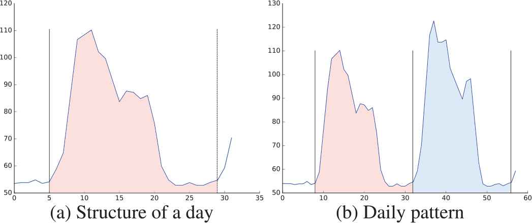
Time series of hourly consumption.
3.1.1. Data processing
Noise is one of the characteristics that is inherent in practically all nonsynthetic datasets. In this particular case, negative values and consumption data were found to be too large in view of the consumption being recorded by a meter. To mitigate this effect, the first step is to replace all hourly observations whose recorded consumption is negative because this constitutes a failure in the meter reading that is easily detectable. At this point, two options were considered: either eliminate the consumption for that hour or replace its value. Bearing in mind that a day has 24 hours, if one of the hours is eliminated, then this means that this day will no longer be complete and, therefore, the remaining hours that are valid in principle will have to be discarded, thus dispensing with a day of consumption. If this situation occurs with a certain frequency, then there is the risk of losing too many data that are valid a priori due to an anomalous observation, which could make it difficult to generate the target groups; that is, G0 and G1. Consequently, we consider that the best option is to replace these wrong observations at the time of capturing consumption, by a value that has a minimum incidence when it comes to grouping data to constitute Mi models. Because the starting data is a negative value, its replacement by a null value (zero) should be the least error to enter at thconstitute the day, which only serves to maintain the range of 24 hours needed without adding any value.
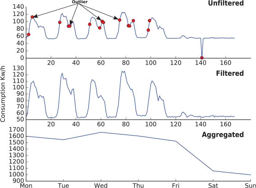
Detecting and replacing negative consumption data is a technique that can be applied to each meter in a trivial way; however, as has already been introduced, it is not the only applicable technique. In addition to negative values, each meter may have recorded values where consumption is very high, depending on the type of activity carried out by the building that is monitoring its consumption or the season of the year to which it corresponds. This type of observation can also lead to errors when calculating the consumption of the day, obtaining the same problem as the negative consumption values. Therefore, it is necessary to mitigate the effect of these anomalous observations on each meter independently. This is important to point out because the consumption between buildings varies—a value that would be excessive in one building, may be normal in another. Consequently, it is necessary to establish a time interval, in hours, that is small enough to detect only alterations in consumption on dates that are related and is large enough to appreciate such variations. After experimentation, it was concluded that the most suitable period to detect these changes in consumption was 7 days, where each day will contain 24 hours of consumption in the interval [5:00 am, 4:00 am] or 168 hours. On this last data window, a statistical technique called interquartile ranges or IQR is applied to detect anomalous observations, which are replaced by a linear interpolation between contiguous observations because we assume that the consumption recorded at a specific time by a meter will be similar to the consumption recorded near that time.
Figure 2 shows the different transformations that a time series undergoes. In the «unfiltered» view, raw data is displayed as they are captured by each meter. It illustrates the different points that are detected as outliers according to the IQR technique, such as in the daily peaks there is an abrupt decrease in consumption to pick up again (hours 38, 59, 85), or in the hour 140 there is a very far value with respect to the consumption obtained in the near future. In contrast, the «filtered» view shows the same series without these anomalous observations. The valleys that were previously highlighted now appear much softer, in accordance with the consumption that is obtained in near dates, and the peak obtained in the hour 140 is now much closer to how the consumption should have been. Finally, the «aggregated» view shows the aggregation of the filtered time series to obtain the total daily consumption, the latest type being the time series data set used to generate the models. These models will be obtained using the k-means algorithm. Both this and other partition-based algorithms have one common feature: to provide the number of k groups in advance to perform clustering. This section has already demonstrated that the proposed Mi meter models will have two groups, or what is the same, k = 2. Therefore, to justify this decision, in the following section a probabilistic study is carried out whose conclusion is based on the available consumption data. The results will be compared with those produced by a series of heuristic techniques.
Transformation of time series.
3.2. Hyperparameter Tuning for k-Means
The k-means is one of the best-known partitioning algorithms that is used in a wide variety of fields [35] due to its ease of implementation and the quality of the results obtained. However, despite its popularity, it suffers from certain limitations that should not be overlooked. As has already been explained, one is to choose the appropriate k, in addition to the incidence of the initialization process on the quality of the results obtained [36, 37]. A simple technique to try to mitigate this problem is to run the algorithm n times for a k given with different initial partitions, selecting the one that minimizes the sum of squared errors [38]. However, this carries with it the difficulty of discerning whether n is adequate or not. Among the existing variants of k-means, there is the so-called k-means++ [37], which tries to select k centroids randomly, one at a time, with a probability proportional to the squared distance with the nearest centroids already selected. Erisoglu et al. [37] point out that the overall performance is better than k-means pure, both in the quality of the result and in the execution. Consequently, it has been decided to use k-means++ to the detriment of k-means as an algorithm to generate the proposed meter models.
3.2.1. Selection of k
Determining the number of groups (k) enables us to associate a descriptive semantics with energy consumption.
The aim is to achieve a balance between the semantics searched and the error made in the process of clustering. It is well known that the greater the k, the more compact the groups will be and, therefore, the smaller the error will be. However, a high value of k does not always bring greater meaning to the final result. Figure 3 shows the distribution of aggregate consumption per day of the week for a full month of three consumption meters, whose identifiers (id) are 1, 62, and 95.
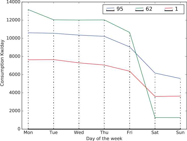
One week’s form of aggregate consumption per day.
At first, we can see a pattern that is repeated throughout the week: a period where consumption is accentuated, drawing a «crest», followed by a «valley» where it decreases to a point where consumption is quite flat and there are no great variations. This suggests that a k = 2 can provide an adequate consumption categorization to the form described by the series. To confirm this hypothesis, let us consider the generation of two groups, with k = 2, where G0 will refer to the categorization of consumption of no activity, and G1 to that of activity. Let W the set of all working days:
Also, consider the following set of conditional probabilities:
To determine the effectiveness of the premise of Equation (8), we are going to use the result of the clustering of one of the meters shown in Figure 3, Meter 62, whose distribution of days per cluster is shown in Table 2. Therefore, the probability that the activity consumption (W) will be in the first group (G0) will be
| Monday | Tuesday | Wednesday | Thursday | Friday | Saturday | Sunday | ||
|---|---|---|---|---|---|---|---|---|
| G1 | 34 | 35 | 34 | 32 | 28 | 1 | 1 | 165 |
| G0 | 11 | 10 | 11 | 13 | 17 | 44 | 44 | 150 |
| 45 | 45 | 45 | 45 | 45 | 45 | 45 | 315 |
Distribution of days per group.
The remaining probabilities are listed in Table 3. Based on the results, we can conclude that as [P (W/G0) < P (H/G0)] and [P (W/G1) > P (H/G1)], our premise is fulfilled and, therefore, our initial hypothesis about the assumption of the number of groups to choose is valid.
| P (W/G0) | P (H/G0) | P (W/G1) | P (H/G1) |
|---|---|---|---|
| 0.413 | 0.586 | 0.987 | 0.012 |
Conditional probabilities.
However, this conclusion has only been shown to be valid for one of the meters. Therefore, we are going to extend our hypothesis Equation (8) for all available consumption meters, which in this case amounts to a total of 97. Let
It is worth noting that mathematical expectation will be estimated through arithmetic mean. So, as in the previous case, to determine its validity, we will make use of the result of the clustering for each of the consumption meters, where a subset of the probabilities already calculated can be seen in Table 4. For example, following the three meters shown in Figure 3, for Meter 1, we have P (W/G0) = 0.148 is less than P (H/G0) = 0.852, and that P (W/G1) = 0.960 is greater than P (H/G1) = 0.040, conditions necessary and sufficient to confirm the hypothesis for selecting two groups. The same applies to Meter 95.
| Meter | P (W/G0) | P (H/G0) | P (W/G1) | P (H/G1) |
|---|---|---|---|---|
| 0 | 0.319 | 0.681 | 0.972 | 0.028 |
| 1 | 0.148 | 0.852 | 0.960 | 0.040 |
| 2 | 0.324 | 0.676 | 0.972 | 0.028 |
| 3 | 0.422 | 0.578 | 0.969 | 0.031 |
| 4 | 0.459 | 0.541 | 0.993 | 0.007 |
| 5 | 0.452 | 0.548 | 1.000 | 0.000 |
| 6 | 0.309 | 0.691 | 0.972 | 0.028 |
| … | ||||
| 90 | 0.415 | 0.585 | 0.969 | 0.031 |
| 91 | 0.363 | 0.637 | 0.924 | 0.076 |
| 92 | 0.392 | 0.608 | 0.970 | 0.030 |
| 93 | 0.381 | 0.619 | 0.970 | 0.030 |
| 94 | 0.324 | 0.676 | 0.972 | 0.028 |
| 95 | 0.289 | 0.711 | 0.973 | 0.027 |
| 96 | 0.000 | 1.000 | 1.000 | 0.000 |
Subset of probabilities.
Thus, the mathematical expectation that the activity consumption (W) will be in the first group (G0) will be of
The remaining expectations are shown in Table 5, where the new extended hypothesis Equation (11) is also fulfilled for the total of consumption meters and, therefore, we can conclude the number of groups we had assumed explains the semantics that we have defined.
| 𝔼 [P (W/G0)] | 𝔼 [P (H/G0)] | 𝔼 [P (W/G1)] | 𝔼 [P (H/G1)] |
|---|---|---|---|
| 0.359 | 0.641 | 0.928 | 0.072 |
Probabilities of expectations.
Through this probabilistic study, it has been demonstrated that the initial hypothesis of categorizing consumption data into two groups with which to generate the Mi meter models is adequate. To reinforce this conclusion, we will check if we obtain the same conclusions using two of the most widely used heuristic techniques in the literature [5, 39–43], gap technique [44] and silhouette [45]. Finally, we draw the same conclusions. To carry out this test, we compare the results obtained by each of these techniques applied on the same three consumption meters as in the previous case: 1, 62, and 95.
Table 6 shows for each k the value achieved by the gap technique (column gap) and silhouette (column sil) for each consumption meter. For example, it can be observed that for Meters 1 and 95, both techniques show that the best possible partition is k = 3 and k = 4, respectively; however, for Meter 62, there is no agreement. Then, based on the results obtained, two problems can be seen:
| 95 | 62 | 1 | ||||
|---|---|---|---|---|---|---|
| k | sil | gap | sil | gap | sil | gap |
| 2 | 0.763 | −16.08 | 0.650 | −14.09 | 0.624 | −14.68 |
| 3 | 0.765 | −15.65 | 0.585 | −14.23 | 0.595 | −14.90 |
| 4 | 0.729 | −15.71 | 0.628 | −13.96 | 0.637 | −14.66 |
| 5 | 0.717 | −15.73 | 0.615 | −14.01 | 0.580 | −14.86 |
| 6 | 0.644 | −15.86 | 0.616 | −14.05 | 0.592 | −14.93 |
| 7 | 0.650 | −15.93 | 0.601 | −14.10 | 0.601 | −14.83 |
Highlighted in bold is the best value obtained for each technique in each meter.
Optimal number of groups.
There is no agreement between the techniques, so the choice of one or the other depends on the expert who is conducting the study.
Having solved the previous problem of choosing the heuristic technique, there is also no consensus when it comes to choosing the k for each consumption meter, which makes it impossible to extrapolate the k obtained for one of the meters to the other meters.
Therefore, the conclusion that emerges is that for a set of heterogeneous consumption time series, as is the case in this paper, trusting in the result of this type of algorithmic solutions is not appropriate because the choice of the k depends on the semantics that we want to assign to the models to be defined, which are shown in the following section:
3.3. Results
To define the Mi meter models, as introduced at the beginning of this section, the consumption data of an educational institution has been gathered from UCLM. Specifically, the period of data available is from 2011 to 2017. Based on this data, we can obtain up to a total of six different Mi meter models, one for each year from 2011 to 2016, because the consumption data corresponding to 2017 will be used to compare the last model (i.e., 2016) with the current consumption level of the organization when generating the associated linguistic summaries. A small sample of the prototypes obtained by the process of clustering for each of the consumption meters is shown in Table 7, which uses the aggregated series to obtain the daily total for each of the available annual periods. It can be observed that some of these periods, such as 2011 or 2012, have no consumption data available and, therefore, there is no generation of groups. This is due to the gradual introduction of consumption meters over the years on the different buildings at UCLM. The only limitation that this implies is the impossibility of using the models of those years for certain meters as reference elements to find if the consumption that we obtained is what was expected.
| Meters | |||||||||
|---|---|---|---|---|---|---|---|---|---|
| 0 | 1 | 95 | 96 | ||||||
G0 | G1 | G0 | G1 | ... | G0 | G1 | G0 | G1 | |
| 2011 | 411.46 | 1006.56 | 420.45 | 791.84 | - | - | |||
| 2012 | 518.99 | 965.09 | 455.23 | 837.04 | - | - | |||
| 2013 | 497.26 | 1044.59 | 603.39 | 1095.65 | - | - | |||
| 2014 | 535.37 | 1064.36 | 487.51 | 954.44 | 261.98 | 793.14 | - | ||
| 2015 | 735.50 | 1748.16 | 498.11 | 1164.04 | 297 | 1965.11 | - | ||
| 2016 | 500.44 | 1215.19 | 570.23 | 1213.66 | 276.31 | 1994.66 | 211.07 | 406.82 | |
Clustering result on each meter i.
As already mentioned, the 2017 consumption data will be used to measure the error made by our models, which will be defined according to the clustering results of 2016. If we use the data from Table 7, then the model definition for Meter 0, for example, will make use of the model definition given in Equation (2), which will be given by M0 = {G0, G1}, where G0 has an associated semantics of no activity, and G1 of activity, whose prototype or most representative consumption is G0 = {500.44} and G1 = {1215.19}, respectively. This gives an actual daily consumption of x, which tells us which group it belongs to by means of a distance measurement. Depending on the associated semantics, we will be able to summarize in linguistic terms the consumption situation of a meter i with respect to the total obtained by the organization, whose definition and generation process will be discussed in the next section.
4. DEFINITION OF ORGANIZATIONAL MODEL
The concept of a meter model Mi has been introduced in the previous section. By themselves, they do not provide enough information to be able to draw conclusions regarding actual consumption being obtained in a given period. For example, if you have an actual consumption of x = 675 KW/day for Meter 0, whose model is determined by M0 = {500.44, 1215.19}, the maximum that you can get is x belonging to the semantic group, but it is not possible to know if this level of consumption is high, moderate, and so on. Therefore, in fact, each Mi meter model is used as a base to establish an organizational model that can serve as a comparative environment for each of the meter models. Thus, an organizational model or metamodel is a model of models composed of each of the meter sub-models Mi, which by means of a linguistic description derived from it, provides a summary of the consumerist situation in which the organization is situated with respect to itself in previous years:
Based on this definition of the organizational model O, conclusions can be drawn about the consumption of each meter model Mi. On the basis of this, a linguistic summary based on fuzzy techniques can be established, which will be discussed below.
4.1. Linguistic Categorization of Each Meter in the Environment O
The organizational model O, for our case study, is defined by
This metamodel O has an associated domain corresponding to the set of prototypes of no activity:
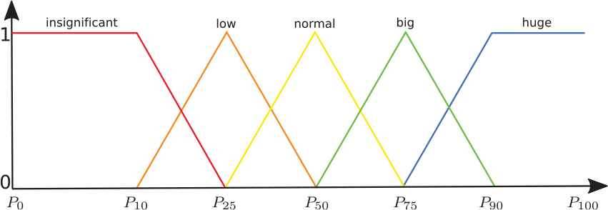
Thanks to the domains of the different groups that make up the organizational model, it is possible to define a characterization of the consumptions obtained by each meter through the calculation of percentiles because they allow us to know the positioning of each meter i in terms of consumption, with respect to the total of the organization. For example, if you have an actual consumption of x = 750 KW/day, and it is known that it is in the 60th percentile (P60) of the organizational model O, then 60% of the meters consume the same or less than x. Therefore, the next step is to define this conclusion or characterization of consumption in linguistic terms to summarize the consumption of each meter i with respect to the organization’s consumption in natural language using the definition of protoforms:
Based on this definition of protoforms, y will be equal to consumption, and the P summary will be defined in fuzzy terms. Now with P, it can be compared the consumption of a meter with the consumption of the organization.
To formalize this summary P, we use a linguistic variable Linguistic variable.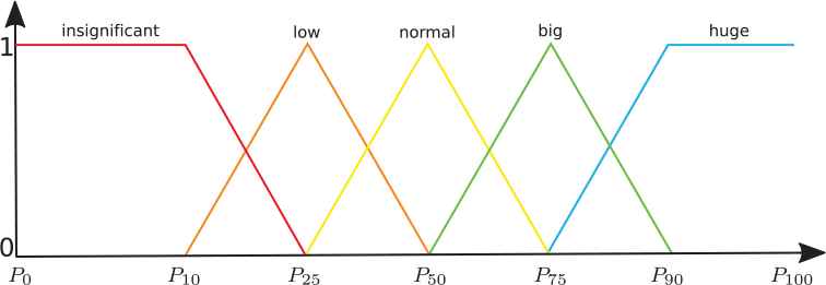
| Label | μ |
|---|---|
| Insignificant | R {P0, P10, p25} |
| Low | T {P10, P25, p50} |
| Normal | T {P25, P50, p75} |
| Big | T {P50, P75, p90} |
| Huge | L {P75, P90, p100} |
Definition of fuzzy sets.
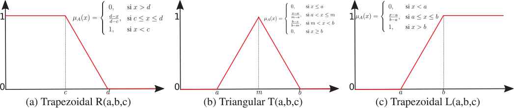
Fuzzy membership functions used.
Once the P summary is formalized, the last step before the linguistic summary can be built is to identify the domain of O to which a given x consumption of a specific i meter belongs to be able to apply the
«Consumption is insignificant, low, normal, big, or huge.»,
«My activity/no activity consumption is insignificant, low, normal, big, or huge.»,
Once the fuzzy set is available, the construction of the linguistic summary would look like consumption is normal. In contrast, if you want to know how the model of Meter 1, M1 behaves with respect to the organization model O, then we must first choose the centroid or prototype cj that we want to compare. Suppose that we choose the centroid in the no activity group (G0 = {570.23}). In this case, it is not necessary to make use of Equation (14) to obtain the semantic group because it is already available with the selection of centroid. As previously, the domain of O on which to apply
As in the previous case, once we have obtained the fuzzy set, the construction of the linguistic summary would be as follows: consumption of no activity is low.
The linguistic summaries that we have seen up to now provide us with the following information for each meter i, during the period of validity of the model: 1. Regarding its actual consumption x, how it behaves as estimated by its model Mi. 2. Regarding your model Mi, how it behaves with respect to the other sub-models of O. However, we lack the necessary information about the error made in the estimation of the meter model Mi to be able to draw conclusions about its goodness; that is, if our model effectively reflects the underlying consumption patterns and, therefore, provides us with adequate conclusions in linguistic terms, or if, in contrast, it tends to be too pessimistic or optimistic in its estimations, drawing incorrect conclusions. Therefore, the following section will propose a mechanism to get a linguistic description of the error made by the models in linguistic terms.
5. LINGUISTIC DESCRIPTION OF THE ERROR
In this section, a framework will be described that will allow us to get the linguistic description of the error of each one of the Mi meter models defined, in addition to the organizational model O. In this way, it is possible to know if the defined model is able to capture the consumption patterns of each meter and of the organization and, therefore, to draw the appropriate conclusions in linguistic terms.
5.1. Description of the Meter Model Mi Error
To carry out the linguistic description of the error of each meter model Mi, it is necessary to associate the actual consumption x obtained in an instant of time in each meter i, with the semantic group Gj of the model that best defines it to obtain the error made in the estimation of the model by actual consumption day. This semantic group will be called
In the particular case that we are dealing with, two semantic groups (k = 2),
| Label | μ |
|---|---|
| No activity | R {0, G0, G1} |
| Activity | R {G0, G1, G1 + G0} |
Fuzzy sets over Mi.
Note that while in Equation (16),
If ϵ > 2σ, then we have predicted a higher consumption than the real one and, therefore, it is overestimated.
If −2σ≤ϵ≤2σ, then we have predicted a consumption that is in line with the real one and, therefore, it is adequate.
If ϵ < −2σ, then we have predicted a lower consumption than the real one and, therefore, it is underestimated.
It is worth noting that with the application of Equation (17), because
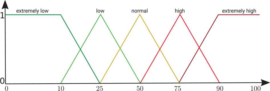
With the ϵ error made by each real consumption x, the interest now focuses on categorizing the relevance of this error in terms of the meter model Mi—that is, if it is placed in the defined margins as adequate or if it is placed in the 5% of the remaining observations—to obtain a linguistic description that sums up the error of the estimated model. To do this, we will use the same linguistic variable
| Label | μ |
|---|---|
| Insignificant | R{0, 10, 25} |
| Low | T{10, 25, 50} |
| Normal | T{25, 50, 75} |
| Big | T{50, 75, 90} |
| Huge | L{75, 90, 100} |
Fuzzy sets on the goodness of the model.
In this case, the domain will be given by the number of observations (errors) that fit into each category described above, according to the following formula:
Given that there are three categories—overestimated, adequate, and underestimated—a linguistic description will be obtained for each, in addition to a global one that summarizes briefly and concisely if our model is still valid for the actual consumption obtained in the current period. For example, in Table 11 you can see the number of errors in each category for Meter 0 with the associated membership of each label defined by the linguistic variable
| Overestimated | Adequate | Underestimated | ||||
|---|---|---|---|---|---|---|
| Lj | μ | Lj | μ | Lj | μ | |
| 1 | 0 | 1 | Insignificant | |||
| 0 | 0 | 0 | Low | |||
| 9% | 0 | 91% | 0 | 0% | 0 | Normal |
| 0 | 0 | 0 | Big | |||
| 0 | 1 | 0 | Huge | |||
Number of errors per category of the Meter 0.
«The model is underestimating the consumption in an insignificant way.»
«The model is adequate in a huge way.»
«The model is overestimating the consumption in an insignificant way.»
To obtain the linguistic description that summarizes in a global way the error made by the meter model Mi, we keep the one whose Lj is maximal. In this case, it would be «The model is adequate in a huge way.»
The indicator to know if our model begins to suffer failures in the estimation of consumption, is determined by the category and the P linguistic summary associated to the description. This means that if the model is underestimating or overestimating consumption, we must look at the value of P to get an accurate conclusion. Thus, if the linguistic label associated with P is less than normal, then we can assert that the linguistic descriptions of the error provided are accurate; otherwise, the model should be updated. Until now, a framework has been established to get a linguistic description of the error made from each meter model present in the organizational model; however, nothing is known about the error made by the latter. Consequently, the following section will extend the concepts presented here so that they can be applied in the organizational model O.
5.2. Description of the Organizational Model O Error
The concepts seen in the meter models can be extended to determine the goodness of the organizational model O. To reach this goal, each category must be aggregated: underestimated, adequate, and overestimated for each meter model Mi that makes up the metamodel O and we must apply the same
Table 12 shows the error made in each meter model by category, including their aggregation according to Equation (20).
| Meter | Lover | Ladequate | Lunder |
|---|---|---|---|
| 0 | 9% | 91% | 0% |
| 1 | 4% | 96% | 0% |
| 2 | 5% | 95% | 0% |
| 3 | 12% | 88% | 0% |
| 4 | 14% | 82% | 4% |
| 5 | 7% | 93% | 0% |
| 6 | 13% | 87% | 0% |
| … | |||
| 90 | 10% | 90% | 0% |
| 91 | 0% | 61% | 39% |
| 92 | 9% | 91% | 0% |
| 93 | 20% | 80% | 0% |
| 94 | 17% | 83% | 0% |
| 95 | 13% | 87% | 1% |
| 96 | 23% | 77% | 0% |
| 9.35% | 87.14% | 3.55% | |
Highlighted in bold is the best value obtained for each technique in each meter.
Number of errors per category of each Mi.
The memberships of each error aggregated by category, «The organizational model is underestimating consumption in an insignificant way.» «The organizational model is adequate to consumption in a huge way.» «The organizational model is overestimating consumption in an insignificant way.»
| Overestimated | Adequate | Underestimated | ||||
|---|---|---|---|---|---|---|
| μ | μ | μ | ||||
| 1 | 0 | 1 | Insignificant | |||
| 0 | 0 | 0 | Low | |||
| 9% | 0 | 87% | 0 | 4% | 0 | Normal |
| 0 | 0.2 | 0 | Big | |||
| 0 | 0.8 | 0 | Huge | |||
Number of errors by category of organizational model O.
We highlight the use of the term organizational to distinguish the linguistic description of the O metamodel from those of each of the Mi meter models that make it up. Again, as in the previous case, the protoform that summarizes in linguistic terms the error made by the organizational model O will be given by that «The organizational model is adequate to consumption in a huge way.»
Throughout this section, a method has been suggested to evaluate each proposed model using fuzzy linguistic summaries. The use of fuzzy sets for their definition offers the possibility of working with little defined limits, so that the conclusion derived from them can be used with some degree of membership of several of these sets. When this is the case, the linguistic summaries based on the protoforms presented in the Section 2 are not sufficiently expressive to highlight this situation. Therefore, in the following section, we introduce a new concept of extended summary that allows us to draw conclusions in linguistic terms whose degrees of fuzzy membership are not very marked.
6. EXTENDED LINGUISTIC SUMMARIES
To reflect a case study in which classic protoforms do not provide enough capacity to capture the semantic hints of a given consumption situation, Table 14 provides a comparison of the membership to the fuzzy sets defined over the linguistic variable of Figure 6 of the same day of actual consumption for two different meters: 0 and 96.
Linguistic variable.
In Meter 0, we have very marked membership levels to the two groups involved (normal and big), so the linguistic summary «consumption is big» provides us with a conclusion that does not give rise to doubt. However, the same does not apply to Meter 96. In this case, we have two sets whose memberships are very close (low and normal). If we were to follow the operation described above, then the most appropriate linguistic description would be «consumption is normal». However, linguistic summaries must be expressive enough to avoid masking information that leads to inaccurate conclusions, as would be the case here.
| Label | Fuzzy membership (μ) | Meter |
|---|---|---|
| Insignificant | 0 | 0 |
| 0 | 96 | |
| Low | 0 | 0 |
| 0.455 | 96 | |
| Normal | 0.003 | 0 |
| 0.544 | 96 | |
| Big | 0.996 | 0 |
| 0 | 96 | |
| Huge | 0 | 0 |
| 0 | 96 |
Comparison of memberships in meters.
To try to capture this idiosyncrasy through linguistic summaries, we propose a modification of the protoforms shown in Section 2:
This extended summary is able to model the linguistic description in terms of two linguistic labels with a nexus that provides the appropriate semantics. Returning to the example of Meter 96, if we use this extended summary, then the linguistic summary would be described as follows: «consumption is being normal close to low.»
Thus, the protoform of Equation (1), making use of this extended summary P′, will, respectively, be defined as
The criteria to determine whether the addition of the W quantifier to the P summary is necessary to obtain a description that captures this kind of cases in linguistic terms will be given by a membership threshold δ associated with each fuzzy set, so that: if the membership value μ of a consumption element x is lower than this threshold, for example, δ = 67%, then it is necessary to use an extended summary P'; otherwise, a summary P is enough.
7. EXPERIMENTAL RESULTS
In this section, we will show the expressive capacity provided by linguistic summaries when summarizing the state of energy consumption of an organization, the UCLM, at a given moment starting from its model. This allows us to analyze specific situations in a legible and intuitive way with to undertake possible corrective actions.
To support the models, a software prototype has been designed and implemented that enables us to monitor and notify the consumption obtained at different management levels of the institution, such as managers and those responsible for the administration of each building. This prototype has been visually structured in three well-differentiated areas, as can be seen in Figure 7: 1. This enables navigation between the different views generated from the models, and certain aspects of administration and management inherent to the application. 2. This shows the options available to select the time ranges with which the model and consumption are to be confronted, and also the type of aggregation resolved on the data, which at this point, only one aggregation is allowed to obtain daily total consumption, and the fuzzy model that will describe in linguistic terms the behavior of the model. 3. Displays different graphical views based on the defined models. The graphical view shown in the Figure 7 provides an organizational level view of the model’s behavior for a particular consumption day. This view has been resolved by means of a treemap, in which each category, represented as big squared tiles, corresponds to the number of i meters grouped in each fuzzy set defined using the
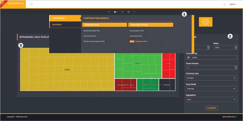
Overview of the software prototype.
Definition of the linguistic variable
Thus, we have also added a new set that is not defined in
In contrast to the proposal to describe the model error that was presented earlier, where three possible cases were defined depending on whether the error committed was adequate, overestimated, or underestimated, and linguistic summaries were constructed that defined the situation of consumption of the organization, in this case we let the fuzzy sets that expose this casuistry according to the membership values obtained in each case. To do this, we use the following equation:
Treemap of consumption on 22 June 2017.
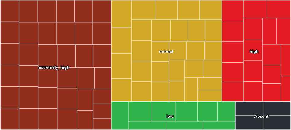
«The consumption of UCLM, with respect its model, is extremely high.»
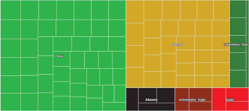
In contrast, we find that on 10 August 2017 electricity consumption was much lower than expected (Figure 10). This day corresponds to the summer holidays period, which is characterized by the closure of all the buildings, so that there is hardly any activity beyond the residual consumption of the meters themselves, the servers, emergency lights, and so on.
Treemap of consumption on 10 August 2017.
In this case, if we apply the linguistic summaries that we defined in the previous section, we can conclude that «The consumption of UCLM, with respect to its model, is extremely low.»
However, if we look at the distribution of meters by category (Table 15), we see that the number of meters that have been categorized with extremely low and low consumption are practically the same. For this reason, the conclusion obtained is not as precise as it should be, since there are meters whose fuzzy membership in these two categories is not very marked. Therefore, for this case, the most appropriate is to use an extended linguistic summary introduced in the previous section, leading to the result «The consumption of UCLM, with respect to its model, is extremely low close to low.»
| Extremely Low | Low | Normal | High | Extremely High |
|---|---|---|---|---|
| 38.14% | 37.11% | 12.37% | 8.25% | 0% |
Distribution of meters by category for 10 August 2017.
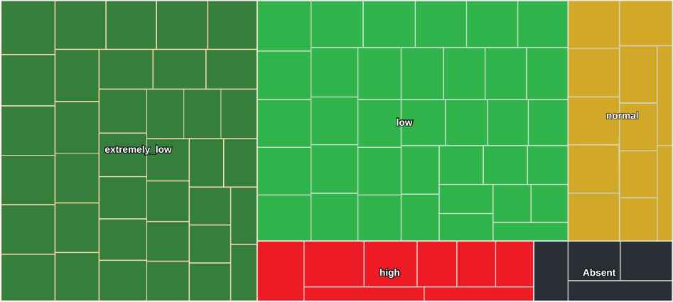
Furthermore, the model behaved best on 4 March 2017, when most of the buildings’ consumption was cataloged as normal (Figure 11). In general, this is the most common trend in the organization for the period 2017. Table 16 shows the distribution of buildings by category for that year. As in the previous cases, if we apply the linguistic summaries defined in the previous section, we can conclude that «The consumption of UCLM, with respect its model, is normal.»
Treemap of consumption on 4 March 2017.
| Extremely Low | Low | Normal | High | Extremely High |
|---|---|---|---|---|
| 3.60% | 23.43% | 42.01% | 17.58% | 9.41% |
Distribution of meters by category of the model O.
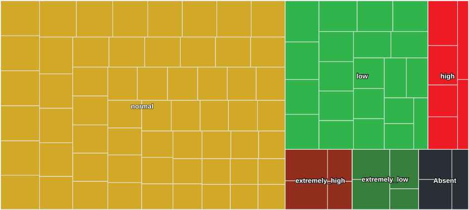
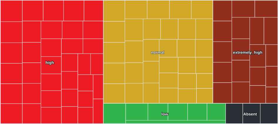
Finally, on 16 January 2017 and 15 April 2017, electricity consumption entries are higher and lower than expected, respectively. The first case (Figure 12) features a day of working activity preceded by a nonteaching period, Christmas, and a week of low work activity, given that it corresponds to a period of examinations, where the activity is limited to certain moments of the day. It is possible that this day concentrated most of the examinations in the different faculties that make up the UCLM, in addition to the use of heating systems due to the low temperatures experienced on a winter day. The second case (Figure 13) corresponds to a nonteaching day because it was in the Easter holiday period, which leads to relatively low consumption. However, it is worth noting that there is enough consumption to not be categorized as extremely low. Finally, by applying the linguistic summaries defined in the previous section, we conclude that in the first case «The consumption of UCLM, with respect its model, is high.»
Whereas, in the second case «The consumption of UCLM, with respect its model, is low.»
Treemap of consumption on 16 January 2017.
Treemap of consumption on 15 April 2017.
8. CONCLUSIONS AND FUTURE WORK
This work proposes a new approach when analyzing and drawing conclusions from a set of time series of energy consumption data, by defining models that summarize the organization’s consumption situation in linguistic terms. This will support decision-making by top managers when undertaking energy policies that contribute to the configuration of sustainable buildings. The definition of these models has been resolved by using cluster techniques. In particular, the k-means algorithm had a good performance and also good quality results. The choice of the number of groups has been based on the semantics that we wanted to associate with the model. In this work, we were motivated to detect consumption patterns (activity), and low or zero consumption (no activity). This allowed us to demonstrate their suitability for the dataset treated using probabilities and mathematical expectations rather than heuristic techniques. We have found that they do not give a uniform criterion of which k is most appropriate when dealing with a set of heterogeneous series. Linguistic summaries based on y is P protoforms have been used for linguistic descriptions, where the summary has been modeled using a collection of fuzzy linguistic variables. The use of fuzzy sets when establishing this summary can lead to situations where it is more appropriate to present it in two labels if the threshold of membership is not very marked. In view of the lack of being able to describe this casuistry through the use of classic protoforms, in this work we propose an extension to model this idiosyncrasy by adding an absolute quantifier. We have also designed and developed prototype software where we support the models shown here, which is currently being used experimentally at the UCLM.
Future work should be aimed at the study of new data preprocessing techniques specific to a set of energy consumption data for electricity. This eliminates noise or mitigates the effect of possible outliers on the quality of the model obtained. To increase the performance of the model, we propose 1. To use the same technique by increasing the number of groups or making a finer segmentation of the identified groups (e.g., taking the data from the activity model (G1) and defining a new submodel). 2. To use different models, such as those based on deep learning techniques. 3. To add more information to the model than just energy consumption data, such as season of the year, weather forecast, building performance calendar, physical characteristics of buildings (m2 , kind of activity), and so on. Furthermore, we think it is possible to incorporate a system of alerts based on linguistic summaries into the model, confronting this proposal with data from other organizations, and develop a big data architecture that is based on microservices to support the definition and manipulation of models.
ACKNOWLEDGMENT
We have received support from the TIN2015-64776-C3-3-R project of the Science and Innovation Ministry of Spain, which is cofunded by the European Regional Development Fund (ERDF).
REFERENCES
Cite this article
TY  - JOUR
AU  - Sergio Martínez-Municio
AU  - Luis Rodríguez-Benítez
AU  - Ester Castillo-Herrera
AU  - Juan Giralt-Muiña
AU  - Luis Jiménez-Linares
PY  - 2018
DA  - 2018/12/17
TI  - Linguistic Modeling and Synthesis of Heterogeneous Energy Consumption Time Series Sets
JO  - International Journal of Computational Intelligence Systems
SP  - 259
EP  - 272
VL  - 12
IS  - 1
SN  - 1875-6883
UR  - https://doi.org/10.2991/ijcis.2018.125905639
DO  - 10.2991/ijcis.2018.125905639
ID  - Martínez-Municio2018
ER  -