1. INTRODUCTION

Is there such a thing as a “History of Curvature?” There certainly are accounts of its history in mathematics [1,2], starting with the geometry of the Ancient Greeks (Euclid of Alexandria’s Elements, ca. 300 bce, developed in the analytic geometry of the 17th century (Réné Descartes [3], Christiaan Huygens [4],¹...) and flowering in modern differential geometry (perhaps starting with Carl Friedrich Gauss’ (1777–1855) famous Theorema Egregium [5]).² For an extensive overview of the field in the mathematical domain see the volumes by Franki Dillen en Leopold Verstraelen [6].

In this paper I’ll take a view that goes against the grain. It doesn’t really fit into the huge and beautiful realm I sketched above.

My main point is that the intuitive notion of “curvature” must have been around much earlier. It should not require formal geometry at all. Such gut level notions necessarily derive from experiences involving perceptions and actions in the real world, not the world of Platonic objects.

But although an earthworm will likely have such experiences,³ it never crosses the border between sentience and sapience. Humans do. It is because humans construct things, both formally, but perhaps even more importantly, with their hands. Thinking with the hands precedes thinking in concepts.⁴

Meaning and understanding derive from what you construct (verum factum est – Giambattista Vico’s Scienza Nova [7]).⁵

2. CURVATURE AT THE GUT LEVEL

You understand curvature when you have constructed it (Figure 1). Biologically speaking, technology is knowledge.

Figure 1

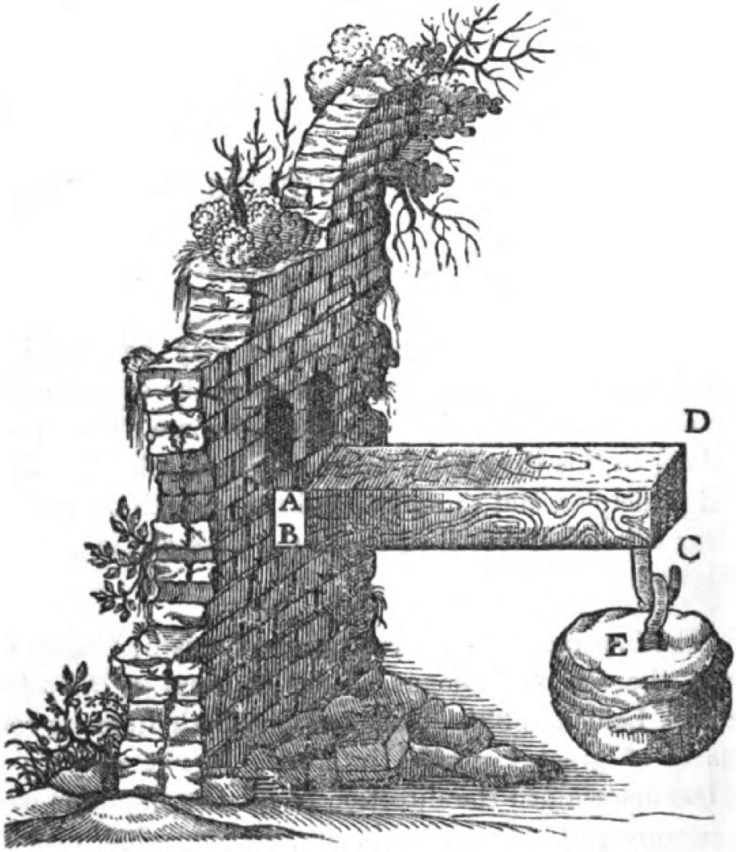
Cantilever beam [Galileo Galilei (1564–1642), Nuove Scienze, [8]]

Reflecting on this in such a way, it occurred to me that the understanding of curvature may have commenced from the invention of the bow and arrow. That takes us back in time much further than the Ancient Greeks, all the way to the transition between the Upper Paleolithic and the Mesolithic [9].

The earliest artifacts date from 17,500 to 18,000 years ago.⁶ From microliths found in the south of Africa one guesses that the origin may go back as far as 71,000 years. After the close of the latest glacial period the use of the bow spread throughout the inhabited world.⁷

A bow⁸ essentially consists of the rigid connection of a pair of cantilever elastic beams (Figure 1) attached to a rigid grip. Sometimes it will be of a single piece (of Yew wood, like the English longbow, say), other times it may be a sophisticated composite involving a complex combination of materials, chosen for their diverse physical properties.

From basic elasticity theory [10] we find that the bending moment M of a cantilever beam is proportional to its curvature κ (“curvature” in the modern sense), one has M = κ EI, where E is a material constant⁹ and I a geometrical constant.¹⁰

There is thus an immediate relation between the visible curvature and the muscular effort involved in loading the beam with elastic potential energy.¹¹ The constants are experienced as the property of the bow as a tool, its “feel.”¹²

The actual physics of the bow is quite complicated [11]. However, the immediate relation between the visible curvature and the muscular effort is what counts here. It renders “curvature” a gut feeling. The construction of the bow turns this gut feeling into a cognitive meaning.

By way of an aside, it might be suggested that the parabolic orbit of the arrow (or a thrown stone, say) might have evoked a feeling for curvature. However, historical evidence pleads against that. Even in the sixteenth century the impetus theory [12], framed by John Philoponus (ca. 530 ce, at Alexandria) was widely adopted (Figure 2).

Figure 2

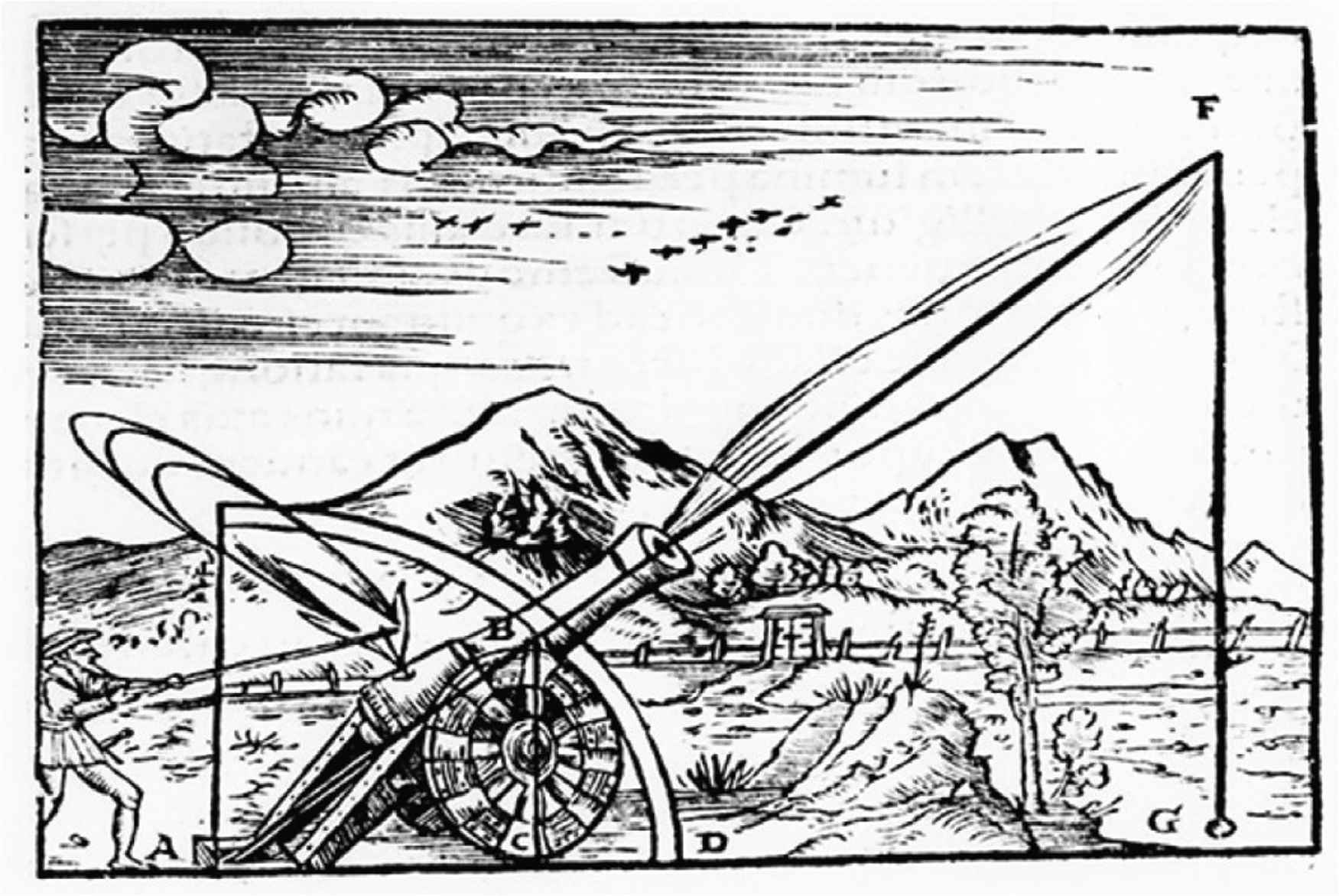
Sixteenth century illustration of the impetus theory of ballistics. Instead of a parabolic orbit, the projectile moves over a straight path. When its impetus is spent, the object regains its “natural motion” and falls straight down. There is no room for curvature. In the 14th century Jean Buridan (he coined the term “impetus”) interpolated a short circular path. A notion of the true shape of the orbit starts with Galileo’s experiments

3. PICTORIAL DEPTH AND THE DUAL NUMBER PLANE

In Figure 3, left the longbow men illustrate the geometry in the plane of the bow. In Figure 3, right we see the personification of Death, standing in a coffin, aim his arrow straight at you. As a spectator, your viewpoint is located in the plane of the bow.

Figure 3

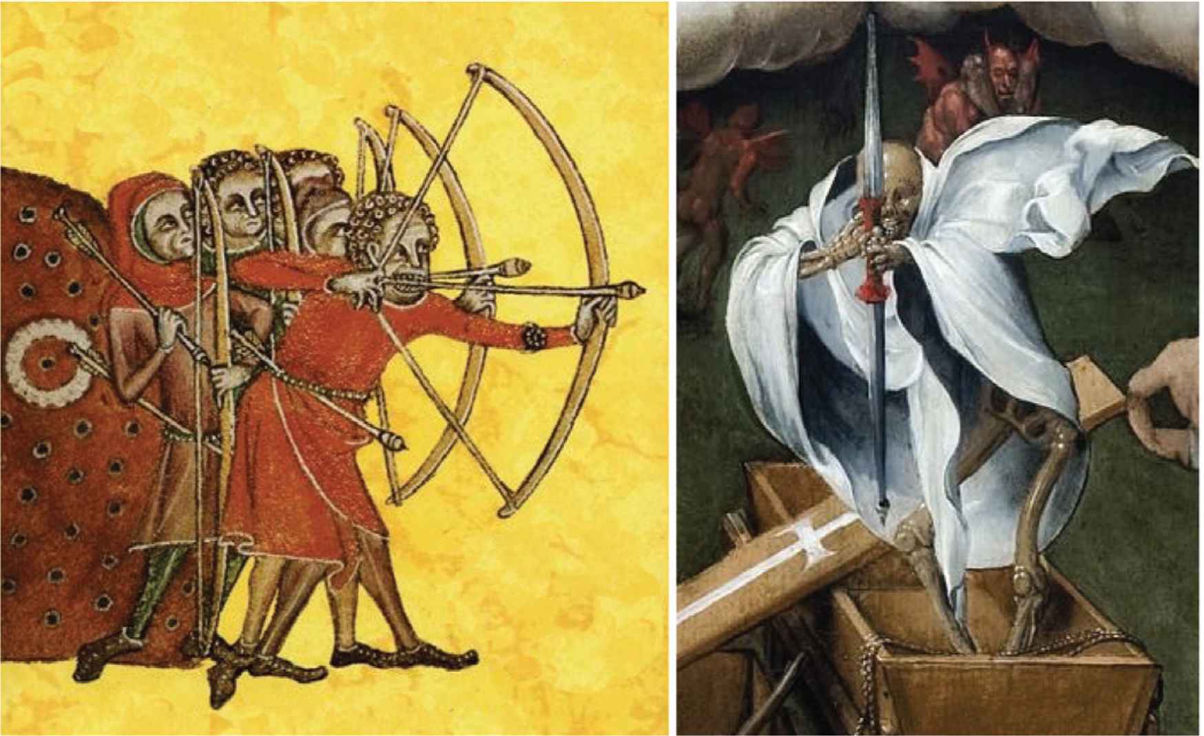
(Left) longbow men, from the Luttrell Psalter, ca. 1325–1335 (British Library). (Right) Hermann Tom Ring (1521–1596), Triomf van de dood, centre panel of a triptych, ca. 1550 (Museum Catharijneconvent, Utrecht.)

This suggests that – geometrically speaking – we might describe the configuration in planar geometry. In the illustration of the longbow men this is the Euclidean plane. In Hermann Tom Ring’s painting the plane has degenerated into a vertical line.

In order to get to see the plane of the bow, you might be inclined to take a side view of the painting. But this does not work! As you step aside Death is still aiming at you [13]. Indeed, Death aims at all spectators in the space before the painting.¹³

I know from experience that it is an eerie feeling to be Death’s target when standing anywhere in front of this remarkable work. It must have made a deep impression on people at the time (mid 16th century). Death never misses!

Apparently, the plane of the bow wielded by death is not our trusty Euclidean plane. The reason is that the physical cause of death is a simultaneous order of pigments distributed on a wooden panel by the painter. The figure of death that you are visually aware of only exists in the mind.

The lost dimension is known as “depth” and it is ontologically distinct from the dimensions that span the picture plane [14–17]. The reason is that all points on a ray through the viewing point¹⁴ are projected on the same retinal location.

The physics needed here is Euclid’s (Euclid of Alexandria, ca. 300 bce) Optics, which is essentially a geometrical information theory of optics [18].

The relevant geometry is the plane spanned by one dimension that has a parabolic metric and one that has an isotropic metric, often known as the “dual number plane.” [19–24].

The dual numbers¹⁵ are complex numbers of the form x + εy, where the complex unit is defined by ε² = 0 ∧ ε ≠ 0. Notice that ε∈𝕉, for it is neither zero (by design), nor positive or negative (because each would imply ε² > 0, which is false).

Intuitively, ε is so small you cannot even see at which side of zero it lies. That makes this geometry the natural model of vision. Euclid might have been the first to join the band wagon as he understood the ontological cleft between the dimensions.

Perhaps surprisingly, the whole depth dimension (an infinite line) is squashed into the infinitesimally thin layer of the picture plane! The mind does not need string–theory to sneak in an additional dimension (depth).

Consider the bow of the Death in the dual plane. It would be 1/2εκu², where the centre of the grip of the bow was placed at the origin. The constant κ would be the “curvature” of the bow, the coordinate u the vertical dimension and the depth the “dual part” 1/2κu².

In this geometry one defines the (signed) distance between z₁ = x₁ + εy₁ and z₂ = x₂ + εy₂ as ||z₁ − z₂||= x₁ − x₂ and – in case x₁ ≡ x₂ – the “special distance” (also signed) y₁ − y₂. One also defines the angular metric through the slope of 1 + εy as y [thus 1 + εy is the dual plane version of a protractor (Figure 4)].

Figure 4

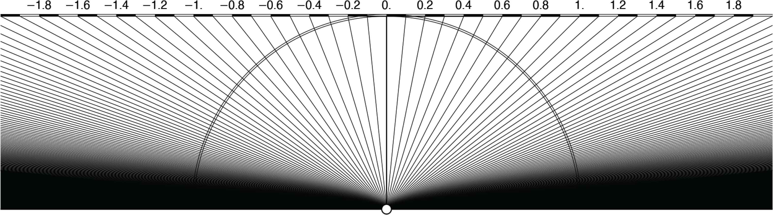
A protractor in the dual plane. The lines are drawn at equal angular increments, their slopes range from minus to plus infinity. The circle shows up the difference with the Euclidean angles. The circular protractor can be completed to a full circle, but the dual slopes are not periodic. The angle metric is the same as the distance metric – rendering this geometry much simpler than Euclidean geometry

Using the conventional definition, the bow is a “circle” in the dual plane, for the slope of the tangent line varies proportional to the arc length (Figure 5). The coefficient of proportionality is the “curvature” κ.

Figure 5

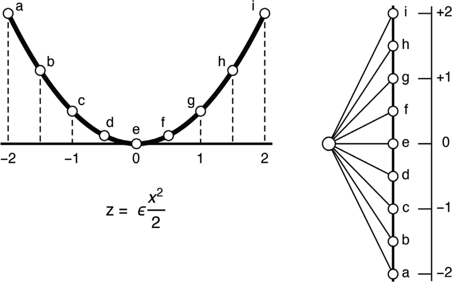
The curve z = εx²/2 represents the circle. The slope at x is x, thus a fixed step along the line implies a fixed step in the angle. That is one definition of a circle

The curve 1/2εκu² is an example of a circle as a curve of constant curvature (Figure 6).¹⁶

Figure 6

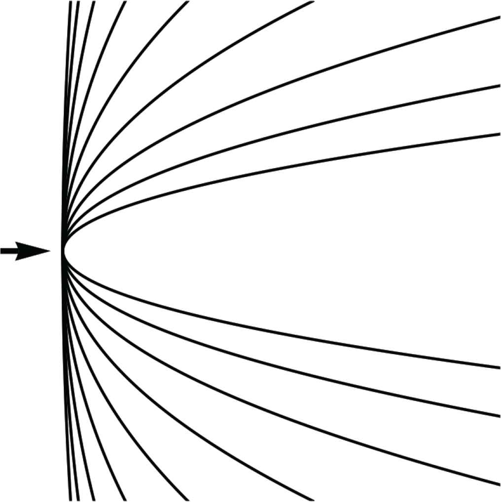
Here the viewing direction is indicated by the arrow. I have drawn a number of circles (curves of constant curvature), the curvature increasing by factors of two. The highest curvature is too much for a bow

The circle of the bow has essentially all of the familiar properties of the Euclidean circle. We compute its curvature as the dual part of d2du2(1/2εκu2)=εκ, that is κ.

I introduced the dual plane because the calculation of the curvature of a curve f(s) as κ(s)=d2ds2f(s) is much more convenient than the Euclidean expression.¹⁷

Curvature is simply the dual part of the second order derivative of a curve (Figs. 5 and 6). This is because the whole depth domain is shrunk to infinitesimal thickness, like in the painting. Thus |f′|<<1 and consequently the awkward Euclidean expression simplifies to κ(s) ≈ f″.

“Pictorial space” (the world we “see in”, that is in the mind) is far simpler than “physical space” (the world we move in, to naive people the “real” world).

Notice that we have defined “curvature” as a second order derivative here, that is to say, in “infinitesimal” [25,26] terms.¹⁸ This is not something that would naturally occur to a Cro Magnon hunter, one of my forebears from the Upper Paleolithic, the Last Glacial Maximum, ca. 48,000–15,000 years ago.

Can we get rid of the derivatives? Well, yes, for most practical purposes we could use small quantities instead of the infinitesimals. But let’s break loose of this altogether.

A straight curve collapses to a point when you put your eye on it. That is one way to check for straightness. This was no doubt the way a Cro Magnon hunter would check his arrows. It is important, for curved arrows do not kill rabbits.

Another way is to notice that something straight can be moved in itself, or that it can be applied in many ways to a copy of itself.

One might also understand curvature as the deviation from straightness. The string of a strung bow looks “straight,” that is why it looks “different” from the bow itself, which looks “curved.”

So we may “know” straightness at the gut level. Then things that won’t fit a straight template might be denoted “curved.”

4. HOW TO MEASURE DEVIATION FROM STRAIGHTNESS

In modern terms we would probably quantify the difference in terms of the root mean square deviations. After a simple shift and picking convenient coordinates, we would measure the difference between the shape {x, y(x)} and the template {x, 0}. The variance would be the average of the quadratic deviation y(x)² minus the square of the average of the deviation y(x).

But over what stretch should we compute it? We might leave that choice open for the moment and use a weighting function w(x) that depends upon a scale parameter t (say).

Many weighting functions are equally useful, but there are good reasons (because Δw = w_t, thus w is the kernel of the diffusion equation [27]) to prefer

a form usually associated with Gauss. The weight is peaked at x = 0, extends approximately over the interval (−2t,+2t), and integrates to 1.

We define the mean of a function f(x) as 〈f(x)〉=∫−∞+∞w(x,t)f(x)dx. Then we define the root mean square (or standard) deviation of f(x) for the scale t as

For f(x) = 1/2κx² we find that SDtf=κt2. Thus the curvature is proportional to the root mean square deviation from straightness. The estimate is the same at any point of the bow, which makes sense because the bow is a circle in the dual plane.

A different method is to apply the more complicated weight

Then ∫−∞+∞wxx(x,t)κx22dx=κ . (see Figure 7) Notice that the application of this weighting function is equivalent to finding the second derivative of the weighted shape at the origin [27].

Figure 7

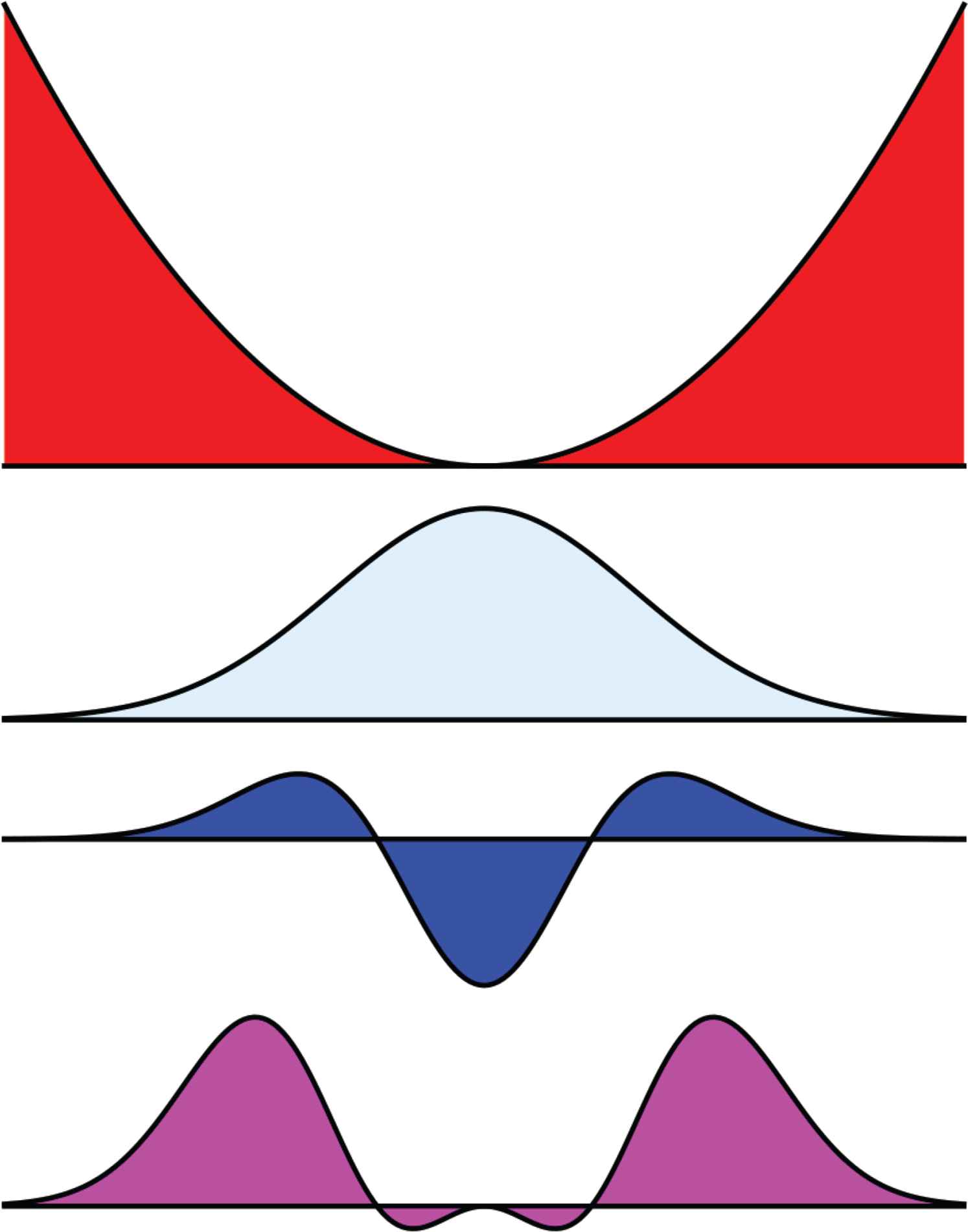
At top the bow is compared with a straight template. The deviations are tinted red. The second row shows a weighting function w(x, t). Notice that its reach (where you see blue) is limited. The third row shows the weighting function w_xx(x, t). The bottom row shows the product of the first and the third row. The total amount of purple stuff is proportional to the curvature at the centre. It is something one may approximately estimate by eye after applying a straight template

Using the diffusion equation we have blown up the infinitesimal domain [26] to the trusty domain of spatial intuition [27].

In either case we have got rid of the pesky infinitesimals. We do not require differentiations. We use only averaging over finite regions (weighted integration). The Cro magnon hunter might do the integration by eye measure – no need to understand the formulas.

Of course, the first estimate also picks up other orders (the second does better). One may consider contributions due to other orders, say a_nxⁿ/n!. For n = 0, 1 they can be nullified by fitting, but orders n > 2 will contribute, although relatively less for small t (their contribution goes by t^n/2) (see [28]).

The standard definition does not have such problems, because it implicitly assumes t = 0 – in itself nonsense from an empirical point of view. Our second method is the remedy for that, it replaces differentiation with integration. The single point (whatever might be meant by that [26]) becomes a blurry finite region.

5. STEPPING A DIMENSION UP, THE DEVIATIONS FROM PLANARITY

Of course, one usually deals with surfaces (as boundaries of volumes) in space, rather than curves in the plane. This is problematic, because our visual field of view is only a topological disk, not a volume. As things in the scene in front of you rotate about general axes this might well lead to surprises.

For instance, in Figure 8, we show an object that may appear (in silhouette) as a triangle, a square, or a circle. Yet it is hardly remarkable, it might well be used as a piece in a board game, for instance.

Figure 8

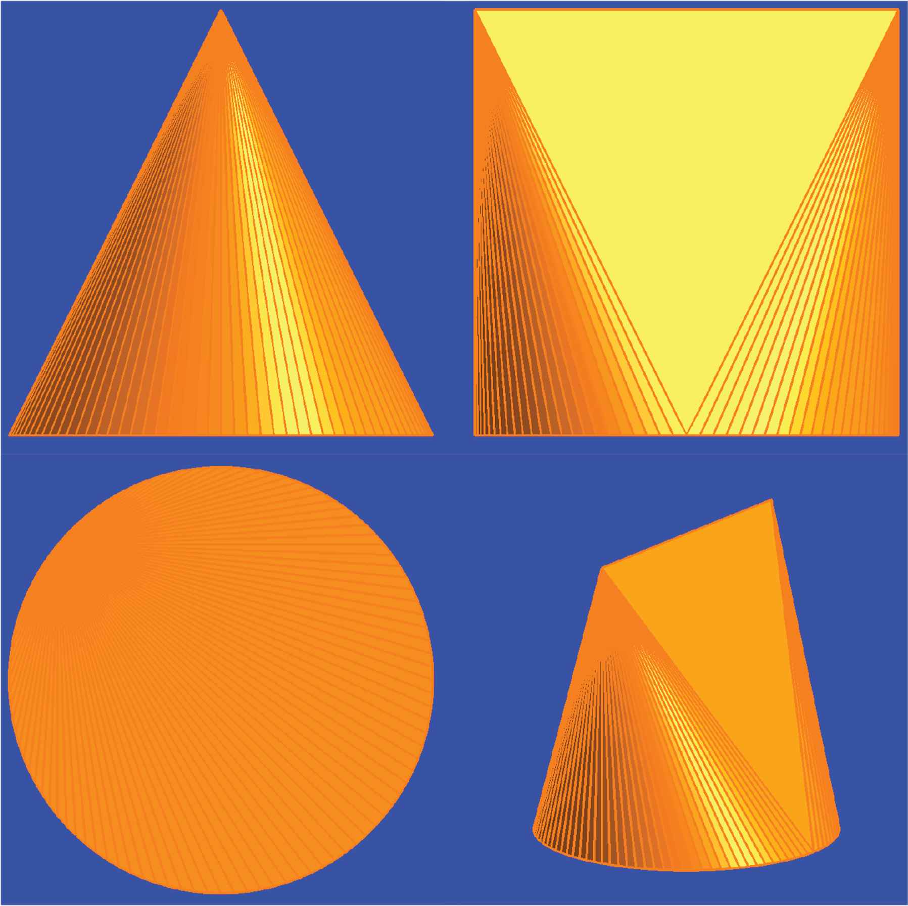
This object has planar parts and regions that are part of right circular cones. In silhouette it might appear as a triangle (or cone), a square (or cube), or a circle (or sphere). Yet it evidently is neither of these

It might be thought that the outline is not informative at all. That is not quite true [29], but close enough. We’re in an awkward situation (optically, that is), when rotations about arbitrary axes are allowed.

The essence of the problem is that so much remains hidden, that is the sad fact that objects have fronts (visible) and backs (not visible, or “optically specified” as people say). The rotations may change the visibility relations.

Here it helps a lot to move to pictorial space. It has three dimensions, two belonging to the picture plane, or the visual field (your choice), whereas the third is generally known as “depth.”

The former two coordinates span a Euclidean plane, whereas the third is to be considered isotropic (remember ε). Now we can do exactly the same things as before.

The surfaces we consider are parameterized as {x, y, εz(x, y)}. We assume z(x, y) to be smooth and of finite slope, thus zx2+zy2<∞. Such surfaces are known as (pictorial) reliefs [30,31].

In pictorial space the metric is ds² = dx² + dy², except for “parallel” points that have zero distance, but different depth. Congruences of the first kind are simply the rotations and translations in the picture plane. In order to avoid unnecessarily complicated expressions we will ignore them.

We only consider congruences of the second kind [32]:

In Figure 9, one has some examples. Of course, there are also mixed transformations, but we ignore them. This is perhaps the simplest setting to consider the curvatures of surfaces.

Figure 9

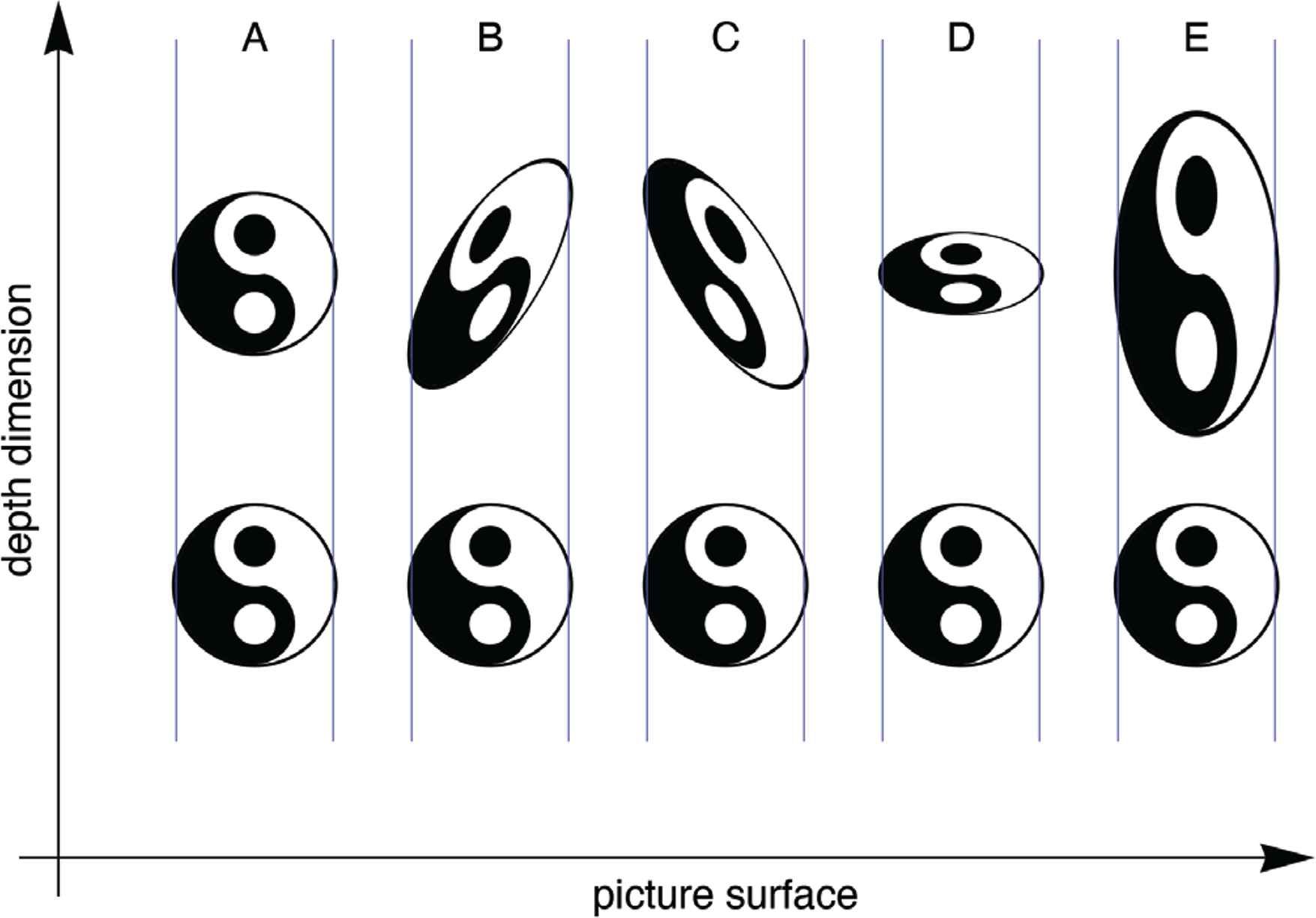
Examples of congruences and similarities, here in the plane y = 0. (You should have no difficulties to imagine the spatial case.) At A I translate the ying-yang figure in depth. (All other examples suffer the same translation, I won’t mention that.) At B I applied a rotation of magnitude 1, at C that rotation has been reversed. At D I show a similarity with modulus 1/2, at E a similarity with modulus 2. Once you get used to these transformations, they look as simple (or actually simpler!) as their Euclidean counterparts

Of the parameters δ, ρ_x, ρ_y and σ, δ is a depth shift. We ignore it because observers have no notion of absolute depth, there is no such a thing.

The pair of parameters {ρ_x, ρ_y} is very relevant. These are the rotations in pictorial space. To the Euclidean eye they look like shears.

The parameter σ really parameterizes a similarity, that is a depth scaling. It is usually non-negative, although depth inversions are known to occur. In this paper we simply assume σ = 1, but in practice it may vary all over the place.

Such congruences and similarities are freely executed as “mental movements” by human observers looking “into” a picture [32].

This can be understood formally from an analysis of the ambiguity left by the optical structure that impinges on the eye [34]. This has also been a topic of research in computer vision [35].

Notice that the rotations of pictorial space do not permit an object to perform a full pirouette. In fact, they cannot change the visibility relations at all. What is seen at one moment is seen at the next, nothing new is ever revealed.

In a portrait painted en face you will never see the back of the head. It is another reason to feel happy in pictorial space, especially if you are a geometrician.

6. THE CURVATURE OF RELIEF

Now we are ready to say what we mean by (local) pictorial shape: It is the invariant of the congruences defined above. It is easy enough to show that this boils down to a slight generalization of the notion of curvature discussed earlier.

We define the Hessian as the curvature:

You will find it easy to check that the Hessian is invariant against the proper motions of pictorial space.

Because z_xy = z_yx, the Hessian is symmetric. As a symmetric matrix it has two real eigenvalues. A congruence of the first kind allows us to change to coordinates such that the Hessian is diagonal. In the two eigen directions we then have exactly the same situation as before in the case of the bow.

Thus there are two novelties. We have a special coordinate system (given by the eigenvectors) and two curvatures instead of one. Since the curvatures are signed (concave or convex with respect to the viewing direction), we obtain three qualitatively distinct cases: convex–convex, concave–concave and convex–concave.

That means roughly, “like the outside of egg shells,” “like the inside of egg shells” and “like a horse’s saddle.” Of course, there are also degenerate cases, such as flat (“like a calm water surface”), flat–convex (“like the surface of columns”) and flat–concave (“like the inside of reeds”).

In the famous catalogue of all conceivable surface shapes, Leon Battista [36] lists all of these (I used his descriptions) except the saddle shapes. This is perhaps remarkable, because Alberti transported himself on a horse, whereas I use a car.¹⁹

Alberti’s first division is divided into three:

Restaci a parlare dell’ altra qualità delle superficie, la quale è (per quasi) come una pelle distesa sopra tutta la faccia della superficie. E questa si divide in tre. Imperocchè alcune sono piane ed uniforme, altre sono sferiche e gonfiate, altre sono incavate e concave.

that is into planar, convex and concave. Then he introduces compound surfaces:

a la superficie composta è quella, che ha una parte di se stessa piana, e l’altra o concava, o tonda, come sono le superficie di dentro delle canne, o le superficie di fuori delle colonne,...

One would perhaps expect the saddles here, but Alberti considers the cylinders (both ruts and ridges) instead. There is no mention of anything like a saddle shape.

Gauss famously related the curvatures mentioned here (called “extrinsic” nowadays) to the metrical relations intrinsic to the surface. That is not a topic of this paper, but it implies that you have to crack a piece of egg shell in order to spread it out flat on the table – it simply “has not enough surface area” for that. Likewise, saddle surface have “too much surface area,” so you need to pleat them in order to force them flat.

What is important here is that Gauss defined two surface measures that each somehow summarizes the two curvatures in the eigen directions κ_1,2 (say). These are the “Gaussian curvature” κ₁κ₁ and the “mean curvature” κ₁ + κ₁. The thing I showed before (Figure 8) has zero Gaussian curvature overall and a non-zero mean curvature only on its conical parts – except for the singular curves and points, that is. The two curvatures are simply the determinant and half the trace of the Hessian.

7. FELICE CASORATI’S DOUBTS

The surface {x, y, x²/2} has mean curvature equal to one and Gaussian curvature equal to zero, surface {x, y, (x² + y²)/2} has mean curvature equal to two and Gaussian curvature equal to one, whereas the surface {x, y, xy} has mean curvature equal to zero and Gaussian curvature equal to minus one. Both mean and Gaussian curvature may turn out to be zero for surfaces that are evidently non-planar.

This evidently disagreed with Felice Casorati (1835–1890) who apparently entertained the gut feeling that curvature should at least be a difference with planarity [37–39]:²⁰

... elle ne saurait satisfaire les hommes en général; car, dans des cas assez ordinaires, elle ne s’accorde pas avec l’idée que tout homme, ayant ou non des connaissances spéciales de mathématiques, conçoit d’une manière plus ou moins vague et pourrait exprimer par les mots courbure d’une surface dans un point.

...

Un géomètre peu soigneux pourrait donc dire, par exemple, que les surfaces cylindriques n’ont pas de courbure, tandis que tout le monde croit qu’elles sont courbes, comme on apprend à les considérer et à les nommer dès les premiers pas dans la vie et dans l’école.

...

Voici donc de quelle manière je propose de mesurer la courbure d’une surface en un point, conformément à l’idée commune, dans les cas où il existe autour du point un fragment de la surface ayant partout un plan tangent.

A “good” curvature measure should only become zero for planes! Thus he defined the “Casorati curvature” as C=(κx2+κy2)/2.

This certainly works, but the way he explains the definition is hardly convincing. All that one may heartily agree on is

C caractérise par sa valeur zéro le manque total de courbure, de mème que la premiere des deux courbures des lignes, que l’on a déjà l’habitude de nommer tout simplement courbure.

Avec cette signification du mot courbure on peut dire:

Si la courbure est nulle en tout point, la surface est plane (la ligne est droite).

Il n’y a que la surface plane (resp. la ligne droite) dont la courbure soit nulle en tout point.

Casorati’s notion did not receive universal acclaim. In a reaction in the same journal Eugène Catalan remarked that to say a sphere and a pseudo-sphere can have “the same curvature” is intuitively absurd [40]. This objection hangs on the very notion of “curvature,” so a short excursion on that topic seems in order.

Surface curvature cannot be completely represented on a linear scale. If one ignores spatial attitude, one ends up with two parameters. (Think of the two principal curvatures, or the Gaussian and mean curvature). Thus the Casorati curvature is in itself insufficient to characterize the nature of the relief (Figure 10).

Figure 10

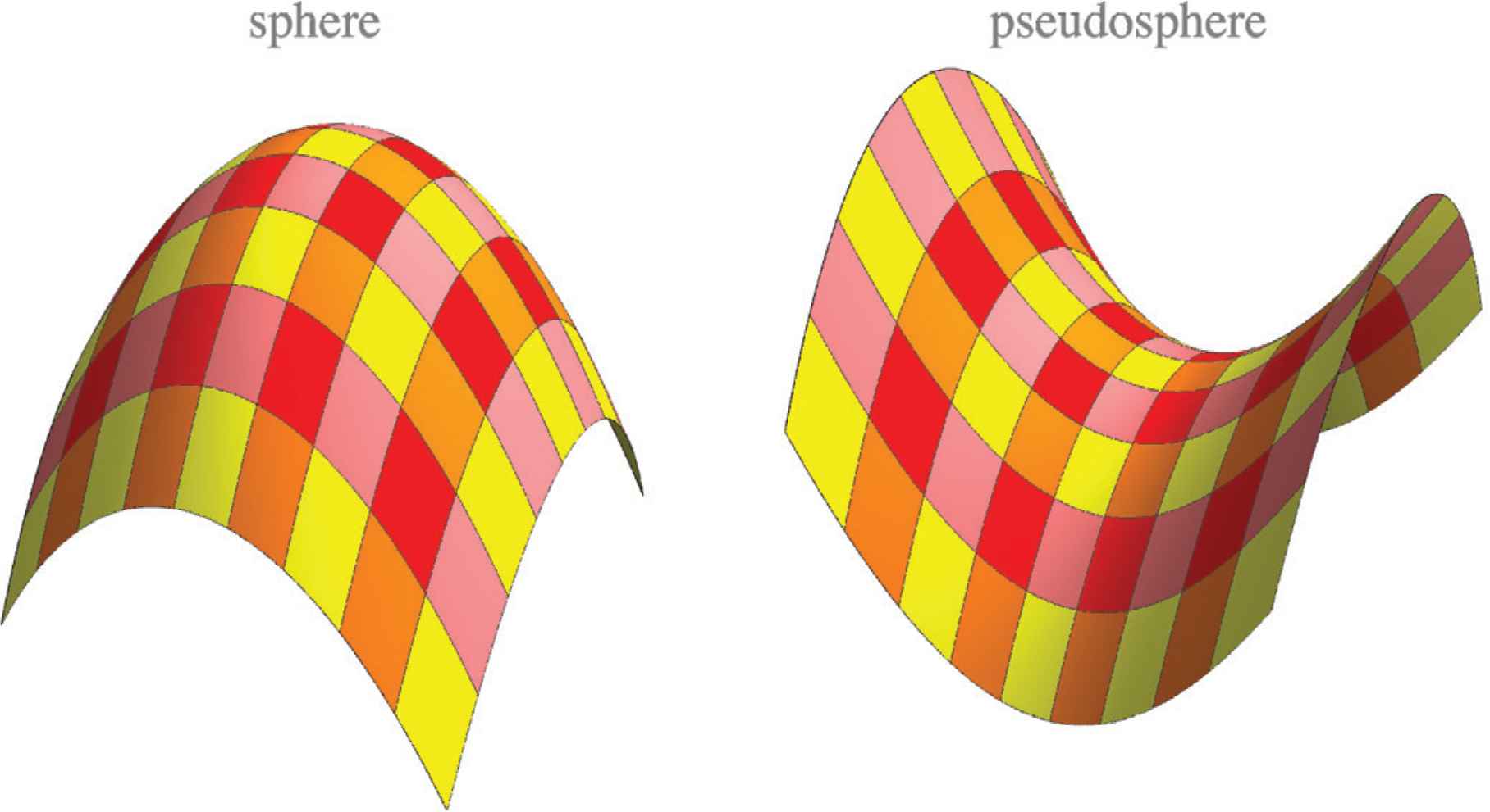
The sphere {x, y, −(x² + y²)} and the pseudosphere {x, y, (x² − y²)}. Both have the same curvature measure (Casorati curvature 4). Yet their “qualities” are very different

However, Casorati correctly identifies a measure of “how much curvature.” This should be completed with a typification. Thus Catalan is right that the (unit) sphere and the pseudosphere appear different, but that does not prevent their curvature measure to be the same.

Unlike the principal curvatures, or the Gaussian and mean curvature, one might desire to characterize surface curvature by way of a quantity and a quality. The Casorati curvature is a natural measure of quantity. The quality might be the ratio of principal curvatures, say. Years ago I introduced a convenient “shape index” based on that notion [33,41]. It distinguishes the (unit) sphere from the pseudosphere, even though their “curvedness” is the same. The shape index is defined on an interval {−1, +1}, whose endpoints represent the umbilics (spheres). Shapes of opposite sign are related by a depth inversion, thus the pseudosphere resides at the origin [42].

In order to show how this works, I write a general quadric in terms of a linear combination of the sphere and the pseudosphere:

(Notice that (x² − y²)/2 and xy are congruent, because (x² − y²)/2 = uv, where u=(x+y)/2, v=(x−y)/2. The coordinate systems {x, y} and {u, v} are mutually rotated over π/4.)

The principal curvatures are κ1=t+r2+s2, κ2=t−r2+s2, thus K = κ₁κ₂ = t² − r² − s², H = κ₁ + κ₂ = 2t. Then the curvedness is C=r2+s2+t2 and I define the shape index as S=t/r2+s2 (that is arctan((κ₁ + κ₂)/(κ₁ − κ₂))).

Since {t, r, s} = {C sin S, C cos S cos2φ, C cos S sin2φ}, the parameters {C, S, 2φ} are special polar coordinates of “shape space.” The Casorati curvature is simply the distance from the origin. Fixing φ factors out orientation, fixing C then leaves us with a semicircle (notice that φ = φ + π) that parameterizes the quality (the shape index).

I continue with a different motivation of the Casorati curvature. In this case the root mean square deviation definition works very well. For using the weight

we find that SDt1/2(κxx2+κyy2)=t2κx2+κy2=2tC. Thus the silly Cro Magnon measure yields Casorati’s preferred answer!

I merely preferred to change Casorati’s curvature into the “curvedness” (κx2+κy2)/2 [33], because then the curvedness of a sphere with principal curvatures κ₁ = κ₂ = κ becomes κ. This might fit the Cro Magnon hunter’s mind better.²¹ It certainly agrees better with my students and many academic colleagues outside the exact sciences.

This is not essentially different from Casorati’s curvature, of course.

8. LEON BATTISTA ALBERTI’S ONTOLOGY AND ARTISTIC INTUITIONS

In order to get some feeling for the convex (or concave) and the saddle-like surfaces, here are some simple observations. The unit sphere (x² + y²)/2 has indeed unit principal curvatures. An arbitrary line in the picture plane x₀ + s cosφ, y₀ + s sinφ can be seen as the projection of

that is on the surface. This is just the rotated and translated unit circle.

Thus all curves on the sphere that project in straight lines are mutually congruent great circles. All have the same curvature, thus surface patches at different locations are perfectly congruent. Indeed, you can move the unit sphere in itself.

Repeating this for the unit “pseudosphere” (x² − y²)/2 (Figure 11), yields

Figure 11

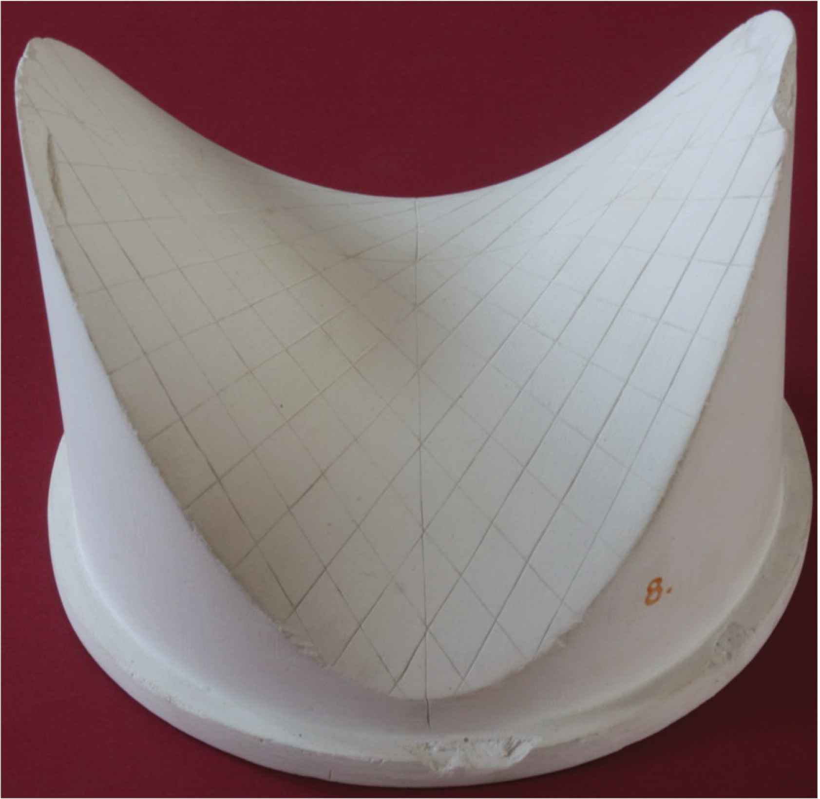
Hyperbolic paraboloid (Modellsammlung, Mathematisches Institut – Universität Göttingen [43]). This is the primordial “saddle surface.” A plaster model that derives from Felix Klein’s activities. (Klein actually held that his mathematics was about the models and not vice versa. He could be more against the grain than I am here.) The lines drawn on the surface show the remarkable “Cartesian net” discussed in the text

This shows that the curvature of curves that project on straight lines is cos2φ. Thus the principal curvatures are ±1, indeed concave and convex.

The lines in the direction φ = ±45° have zero curvature. Consider two of such lines that are parallel in the projection. These lines have different slopes, but they keep constant distance, like a railway track.²² Thus we find two mutually orthogonal families of parallel lines on the pseudosphere (Figure 11).

A Cartesian net of equally spaced lines in two mutually perpendicular directions can be bended into pseudospherical surfaces. Thus we have a Cartesian net on a curved surface! But, of course, any oblique line is curved.

However, to the “Euclidean Eye” such a deformation is not a bending because the “railway tracks” are no longer equidistant.

In mechanics and modern computer science the Casorati curvature (in Euclidean terms) has become known as the “bending energy.”²³ This is related to continuum mechanics, the bending of plates. It immediately calls to mind the example of the bow. Might the experience with elastic deformations apply to higher dimensions (like surfaces)?

Nice as this would be, it is perhaps accidental. Too bad. The primordial curved surface is no doubt the outside of an egg shell. But it is not even possible to bend a flat sheet of paper into an egg shape. The situation is very unlike that in the case of the bow. Here Gauss’ discussion on intrinsic geometry becomes very relevant, as it was not at all for the bow.

In order to forge a flat sheet into some interesting surface the tailor uses cuts, seams and pleats, the cobbler and the brownsmith use extensive hammering to locally change the properties (the metric!) of the plate. Thus we lack the kind of experience we may have in the case of the curvature of beams.

In Euclidean space only spheres and planes can be arbitrarily moved in themselves. If you rub two solids together long enough, using some type of abrasive, they will automatically assume a spherical form, one convex, one concave. This is the time honored way to grind optical lenses. Aspherical surfaces were very hard to produce before the advent of computer controlled grinding machines.²⁴ In order to produce a flat surface one works pairwise on three pieces.

For larger flats, say billiard tables, one has to proceed differently. Frequent testing with straight templates applied at different locations and in different directions is necessary.

The final “flatness” of such surfaces is defined statistically, much as we did in the curvature definition “against the grain.” Such tests and measures are an important part of various technologies. The corresponding literature is completely unrelated to the mathematical literature on curvature.

In the case of surfaces most of our understanding comes from haptic and visual experiences with found objects. Think of eggs, fruits, leaves, stones, landforms and so forth. Alberti was an intellectual who really thought about the topic, but – apart from the degenerate cases with one or two vanishing curvatures – could only come up with concavities and convexities. He completely missed the saddle shapes. Yet saddle shapes are by no means rare. On a Gaussian random surface the saddle-like points are actually in the majority [28]!

Indeed, we have found that even modern Western intellectuals are largely “saddle–blind.” Why might that be?

If you dig for sculptor’s intuitions (they ought to be experts!) you find that the academies tell you to “go for the convexities, the concavities (they probably include the saddles) will take care of themselves!” [44].

Given that the human or animal unclad body [45] has been a major topic for the sculptor since the earliest times (Figure 12), this actually starts to make sense.

Figure 12

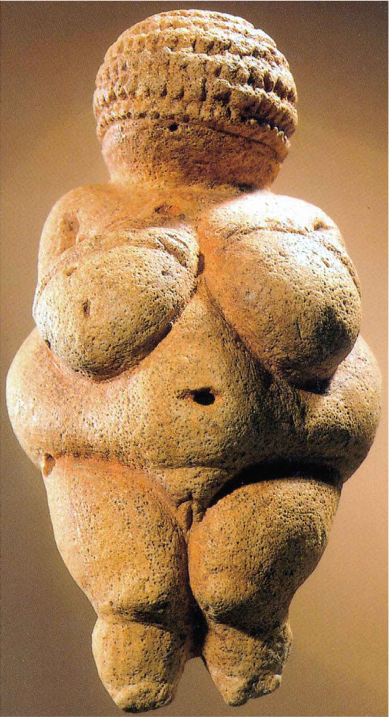
The “Venus of Willendorf” [46] is a small (11 cm) figurine, carved from oölitic limestone with a flintstone scraper and tinted with red ochre. It dates from European Upper Paleolithic (Old Stone Age) starting around 30,000 bce. Notice that it is almost completely made up of convexities, the saddle-like parts having been summarized as sharp V–grooves

The articulation of body surface (I’m not talking about extremities as related to the trunk) is due to the musculature, which is slightly softened by layers of fat and elastic skin. The muscles attach to bones and have their swelling bellies away from the point of attachment. Thus the body surface is governed by dimples (the places where muscles attach to bony crests just below the skin), ruts (the grooves between muscle bodies) and ovoid shapes (the bellies of the muscles).

The result is that the body relief is similar to a bunch of grapes. Benvenuto Cellini (1500–1571)²⁵ likened the treatment by Bandinelli – in an obviously pejorative manner – as similar to a sack of melons put in some corner [47]. I feel he had a point (see Figure 13).²⁶

Figure 13

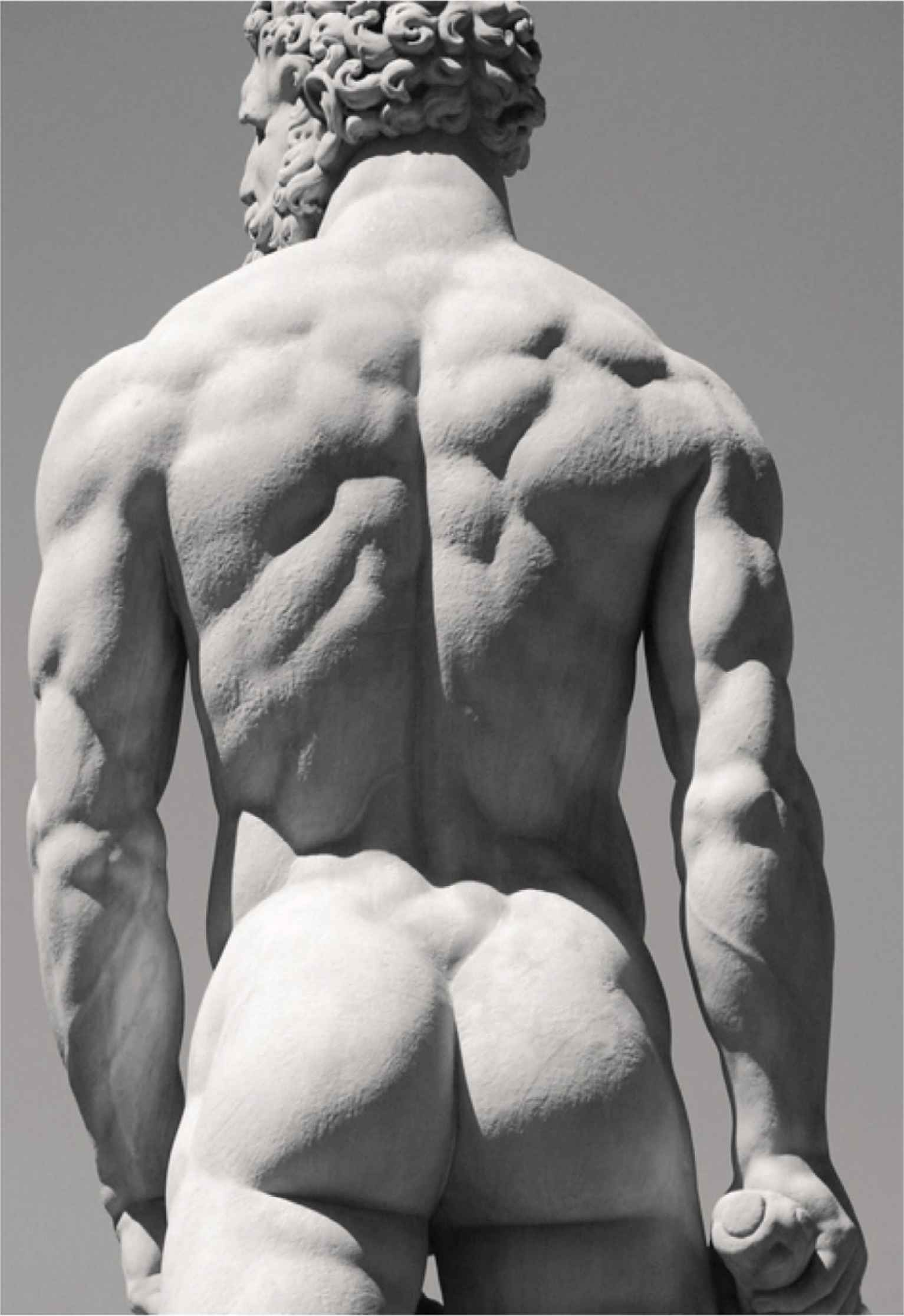
The back of Hercules in the statue of Hercules and Cacus (1530–1534) by Bartolommeo (or Baccio) Bandinelli (1488–1560) at the Piazza della Signoria, Florence, Italy. Notice that Bandinelli’s treatment of Hercules is not all that different from that of the Paleolithic artist. There are almost only convexities meeting each other in (slightly softened) V–grooves

9. MORE TO FOLLOW UP

Another reason for the more than coincidental dominance of convexity is that objects of limited size tend to be convex. One sees this in beach pebbles, where the shapes are due to random abrasion [48].

In organic bodies one has the additional factor that it is good to maximize volume for a given area, as it counteracts drying out. This is obvious in many fruits. Indeed this type of optimality pops up in many physically/physiologically distinct settings (e.g. [49]).

These factors are in no way exhaustive. There are numerous processes that play a role and the biologically relevant costs are diverse too. We tend to be sensitive to this and look with some pleasure on shapes that reflect some kind of intuitive optimum.

So much for a view on curvature that is frankly against the grain. However, I certainly feel that there is plenty of room for further research along these lines.

CONFLICTS OF INTEREST

The author declares they have no conflicts of interest.

ACKNOWLEDGMENTS

The work was supported by the DFG Collaborative Research Center SFB TRR 135 headed by Karl Gegenfurtner (Justus-Liebig Universität Giessen, Germany) and by the program by the Flemish Government (METH/14/02), awarded to Johan Wagemans. Jan Koenderink is supported by the Alexander von Humboldt Foundation. The author is grateful to Andrea van Doorn for many discussions and corrections.