
Implications of Changing the Asymptotic Diastolic Pressure in the Reservoir-wave Model on Wave Intensity Parameters: A Parametric Study
Present address: Centre for Genomics and Child Health, Blizard Institute, Queen Mary University of London, London, UK
- DOI
- 10.2991/artres.k.200603.003How to use a DOI?
- Keywords
- Variation; P∞; wave intensity
- Abstract
Hybrid reservoir-wave models assume that the measured arterial pressure can be separated into two additive components, reservoir/windkessel and excess/wave pressure waveforms. Therefore, the effect of the reservoir volume should be excluded to properly quantify the effects of forward/backward-travelling waves on blood pressure. However, there is no consensus on the value of the asymptotic diastolic pressure decay (P∞) which is required for the calculation of the reservoir pressure. The aim of this study was to examine the effects of varying the value of P∞ on the calculation of reservoir and excess components of the measured pressure and velocity waveforms.
Common carotid pressure and flow velocity were measured using appalanation tonometery and Doppler ultrasound, respectively, in 1037 healthy humans aged 35–55 years; a subset of the Asklepios population. Wave speed was determined using the PU-loop (Pressure-Velocity Loop) method, and used to separate the reservoir and wave pressures. Wave intensity analysis was performed and its parameters have been analysed with varying P∞ between −75% to +75% of its initial calculated value.
The underestimation (up to −75%) of P∞ (with respect to a reference value of 48.6 ± 21 mmHg) did not result in any substantial change in either hemodynamic or wave intensity parameters, whereas its overestimation (from +25% to +100%) brought unrealistic increases of the studied parameters and large standard deviations. Nevertheless, reservoir pressure features and wave speed seemed insensitive to changes in P∞.
We conclude that underestimation and overestimation of P∞ produce different hemodynamic effects; no change and substantially unrealistic change, respectively on wave intensity parameters. The reservoir pressure features and wave speed are independent of changes in P∞, and could be considered more reliable diagnostic indicators than other hemodynamic parameters, which are affected by changes in P∞.
- Copyright
- © 2020 Association for Research into Arterial Structure and Physiology. Publishing services by Atlantis Press International B.V.
- Open Access
- This is an open access article distributed under the CC BY-NC 4.0 license (http://creativecommons.org/licenses/by-nc/4.0/).
1. INTRODUCTION
Incremental changes of arterial blood pressure are determined by forward and backward waves, originated from the heart and from the periphery, respectively. The reservoir-wave theory assumes that the measured pressure consists of two additive components: reservoir (Pr) and “excess” pressure (Pex). This approach was successfully applied by Wang et al. [1] in canine aorta and for the calculation of venous reservoir [2]; then it was extended to any arbitrary arterial location [3,4]. Great differences of clinical and physiological hemodynamic relevant parameters, particularly the size of reflected waves, were reported in a comparison of wave speed and wave intensity analysis determined with and without the reservoir-wave approach [5].
The calculation of Pr requires fitting the diastolic decay of the measured pressure waveform to determine P∞ (asymptotical value) and b (time constant) and there is no consensus over either the value of these parameters or the fitting method for their quantification. Some researchers decided not to fit P∞ but kept it fixed. Specifically, Aguado-Sierra et al. [3] fixed P∞ = 0 mmHg for experimental data and P∞ = 3.2 mmHg (432.6 Pa) for computational data, following Wang et al. [2], who suggested that the asymptotical value is affected by the waterfall effect. Vermeersch et al. [6] calculated the reservoir pressure in the Asklepios population following Aguado-Sierra et al. [3]; however, they found non-physiological values of P∞ with free-fitting and decided to set the asymptotical value to 0 for the entire dataset. A successive study conducted by Aguado-Sierra et al. [4] on human subjects used the same framework but imposed P∞ = 25 mmHg, based on previous work of Schipke et al. [7], who determined the arterial asymptotical value in anesthetized humans under fibrillation/defibrillation sequences.
In a parallel article the effects of varying fitting technique on hemodynamic and wave intensity parameters have been analysed. In this study, we focus on the possible implications of assuming a specific value of P∞. It is hypothesised that different values of P∞ would lead to different reservoir and excess waveforms, affecting hemodynamic and wave intensity parameters. By using a reference value of P∞ and changing it by certain percentage (from −75% to +100%), the comparative analysis was performed.
2. MATERIALS AND METHODS
2.1. Study Group
Details of the Asklepios Study comprising a cohort of middle-aged European participants, can be found in earlier work [8]. Briefly, the subjects were free from manifest cardiovascular disease at study initiation and were randomly sampled from the Belgian communities of Erpe–Mere and Nieuwerkerken. All examinations spanned a timeframe of 2 years and were conducted by a single observer and carried out with a single device. Clinical data, blood samples and hemodynamics measurements were acquired, as explained in the subsequent paragraphs in details.
The entire Asklepios cohort was not used for this study, but a subset of 1037 subjects. Table 1 summarizes the clinical and demographic characteristics of the study group.
| n | Age (years) | Height (cm) | Weight (kg) | SBP (mmHg) | DBP (mmHg) | MAP (mmHg) | HR (bpm) | ||
|---|---|---|---|---|---|---|---|---|---|
| First HD | T | 311 | 38 ± 2 | 171 ± 9 | 73 ± 13 | 127 ± 13 | 74 ± 10 | 96 ± 10 | 63 ± 9 |
| F | 162 | 38 ± 2 | 165 ± 6 | 66 ± 10 | 123 ± 12 | 74 ± 10 | 95 ± 11 | 65 ± 10 | |
| M | 149 | 38 ± 2 | 178 ± 6 | 81 ± 11 | 132 ± 12 | 75 ± 10 | 98 ± 10 | 61 ± 8 | |
| Second HD | T | 262 | 44 ± 2 | 170 ± 9 | 72 ± 13 | 129 ± 14 | 77 ± 10 | 99 ± 11 | 64 ± 11 |
| F | 142 | 43 ± 2 | 165 ± 6 | 65 ± 10 | 126 ± 15 | 75 ± 10 | 97 ± 12 | 66 ± 10 | |
| M | 120 | 44 ± 1 | 176 ± 7 | 81 ± 11 | 133 ± 12 | 79 ± 10 | 101 ± 11 | 61 ± 12 | |
| Third HD | T | 254 | 48 ± 1 | 170 ± 9 | 75 ± 14 | 131 ± 13 | 77 ± 10 | 100 ± 10 | 65 ± 9 |
| F | 120 | 48 ± 1 | 163 ± 6 | 66 ± 11 | 128 ± 13 | 75 ± 9 | 98 ± 10 | 66 ± 8 | |
| M | 134 | 48 ± 1 | 175 ± 6 | 82 ± 11 | 135 ± 13 | 79 ± 10 | 102 ± 11 | 64 ± 11 | |
| Fourth HD | T | 210 | 54 ± 2 | 168 ± 9 | 73 ± 13 | 136 ± 16 | 79 ± 10 | 104 ± 12 | 64 ± 10 |
| F | 107 | 53 ± 2 | 161 ± 6 | 66 ± 10 | 136 ± 18 | 78 ± 11 | 104 ± 14 | 65 ± 8 | |
| M | 103 | 54 ± 2 | 175 ± 6 | 81 ± 11 | 137 ± 14 | 80 ± 9 | 104 ± 10 | 62 ± 12 | |
Values are reported as mean ± SD. DBP, diastolic blood pressure; F, female; HD, half-decade; HR, heart rate; M, male; MAP, mean arterial pressure; SBP, systolic blood pressure; T, total.
Basic characteristics of the study group (n = 1037)
2.2. Protocol
Subjects were asked to lay down in recumbent position, with the neck slightly hyperextended and turned approximately 30° contralateral during carotid scanning. Applanation tonometry and vascular echography were used to acquire blood pressure and flow velocity measurements, respectively. The measurements were not simultaneous, nonetheless acquired during the same vascular examination. The signals were post-processed and aligned using custom-made algorithms Swalen & Khir [9].
2.3. Pressure and Flow Measurements
A Millar pentype tonometer (SPT 301, Millar Instruments, Houston, TX, USA) was used for measuring the pressure measurements and data were recorded at a sampling rate of 200 Hz, continuously for 20 s. Details of the applanation tonometry technique can be found in Rietzschel et al. [8] and the procedure can be summarized in two steps [10]: (a) tonometric tracings were collected from the brachial artery, divided into individual beats, using the foot of the wave as a fiducial marker, then ensemble-averaged. The averaged tracing was successively calibrated using oscillometrically measured brachial systolic and Brachial Diastolic Blood Pressure (DBPb) values as reference markers. Mean Arterial Brachial Pressure (MAPb) was calculated by numerically averaging the curve; (b) tonometry was performed on the common carotid artery, the obtained tracings were ensemble-averaged and calibrated as in step (a), assuming that diastolic and mean pressure values are fairly constant in large arteries, thus using DBPb and MAPb as reference markers. The carotid pressure waveform (P) was scaled accordingly and used in the following analyses.
A commercially available ultrasound system (VIVID 7, GE Vingmed Ultrasound, Horten, Norway), equipped with a linear vascular transducer (12 L, 10 MHz), was used to measure blood flow velocity via Pulsed Wave Doppler, spanning 5–30 ECG-gated cardiac cycles during normal breathing. More details can be found in Rietzschel et al. [8]. The obtained DICOM images were subsequently processed [11] with home-written programs in Matlab (The MathWorks, Natick, MA, USA): maximum and minimum velocity envelopes were detected via morphological operations and averaged to obtain a velocity profile. Single velocity contours (U) were finally obtained from this velocity profile by dividing it into individual cardiac cycles and ensemble-averaging those.
2.4. Data Analysis
Data analysis was performed via custom-made algorithms in Matlab. P and U waveforms were separated into their reservoir and excess components. The reservoir pressure was calculated following Aguado-Sierra et al. [3]:
After the calculation of diastolic Pr (which requires the determination of b,
The complete reservoir waveform is obtained via Equation (1) and the excess pressure from the difference: Pex = P − Pr. Similar analysis held for the velocity components Ur and Uex, where U = Ur + Uex and
2.5. Fitting Algorithm Settings
The length of the fitting window was set to be the entire diastolic period and
| P∞ variation (w.r.t.R) | P∞ value (mmHg) |
|---|---|
| −75% | 12.2 ± 5.3 |
| −50% | 24.4 ± 10.5 |
| −25% | 36.4 ± 15.7 |
| 0% (R) | 48.6 ± 21.0 |
| +25% | 60.8 ± 26.2 |
| +50% | 72.9 ± 31.4 |
| +75% | 85.0 ± 36.6 |
| +100% | 97.2 ± 41.8 |
Values are reported as mean ± SD. w.r.t.R, with respect to the reference value (R).
Actual asymptotical pressure values used in the analysis (n = 1037).
The following hemodynamic parameters were calculated: the maxima of Pr and Pex (Pr max and Pex max, respectively), the time integral of reservoir pressure (PRI) and integral of excess pressure (PEI) curves, respectively (therefore having units of Pa·s) and the maxima of Ur and Uex (Ur max and Uex max, respectively).
Examples of varying waveforms (reservoir and excess, pressure and velocity) with P∞ are shown in Figure 1, with artificially extended reservoir pressure contours displayed in Figure 2 (where the ratios among P∞ values are clearer).
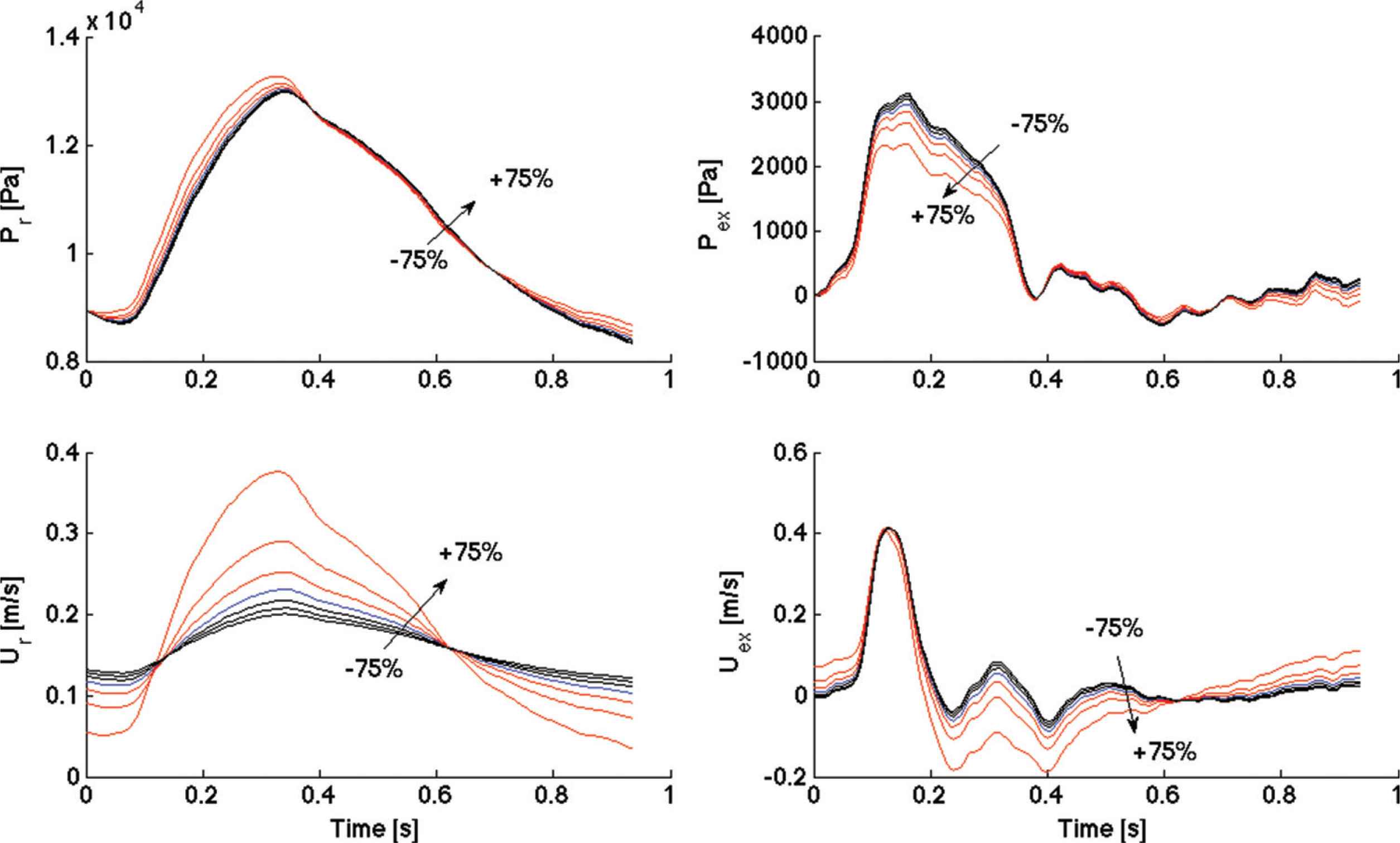
Comparisons of reservoir pressure waveforms (Pr, Top left), excess pressure waveforms (Pex, Top right), reservoir velocity waveforms (Ur, Bottom left) and excess velocity waveforms (Uex, Bottom right) for one subject, among positive (up to +75%) and negative (up to −75%) variations of P∞, with respect to the reference value (R). The +100% variation is not reported because it would alter the scale. An arrow indicates the direction of increasing variation, from negative to positive.

Comparison of diastolic reservoir pressure decay among positive (up to +75%) and negative (up to −75%) variations of P∞, with respect to the reference value (R) for one subject and artificially extended compared to Figure 1. An arrow indicates the direction of increasing variation, from negative to positive.
2.6. Wave Intensity Analysis
Wave intensity analysis was performed on excess waveforms (Pex, Uex) for each subject. Assuming that reflected waves were absent during the early systolic portion of each cardiac cycle [12], the slope of the linear part of the PexUex loop was used to calculate the corresponding wave speed value (m/s) using the following equation:
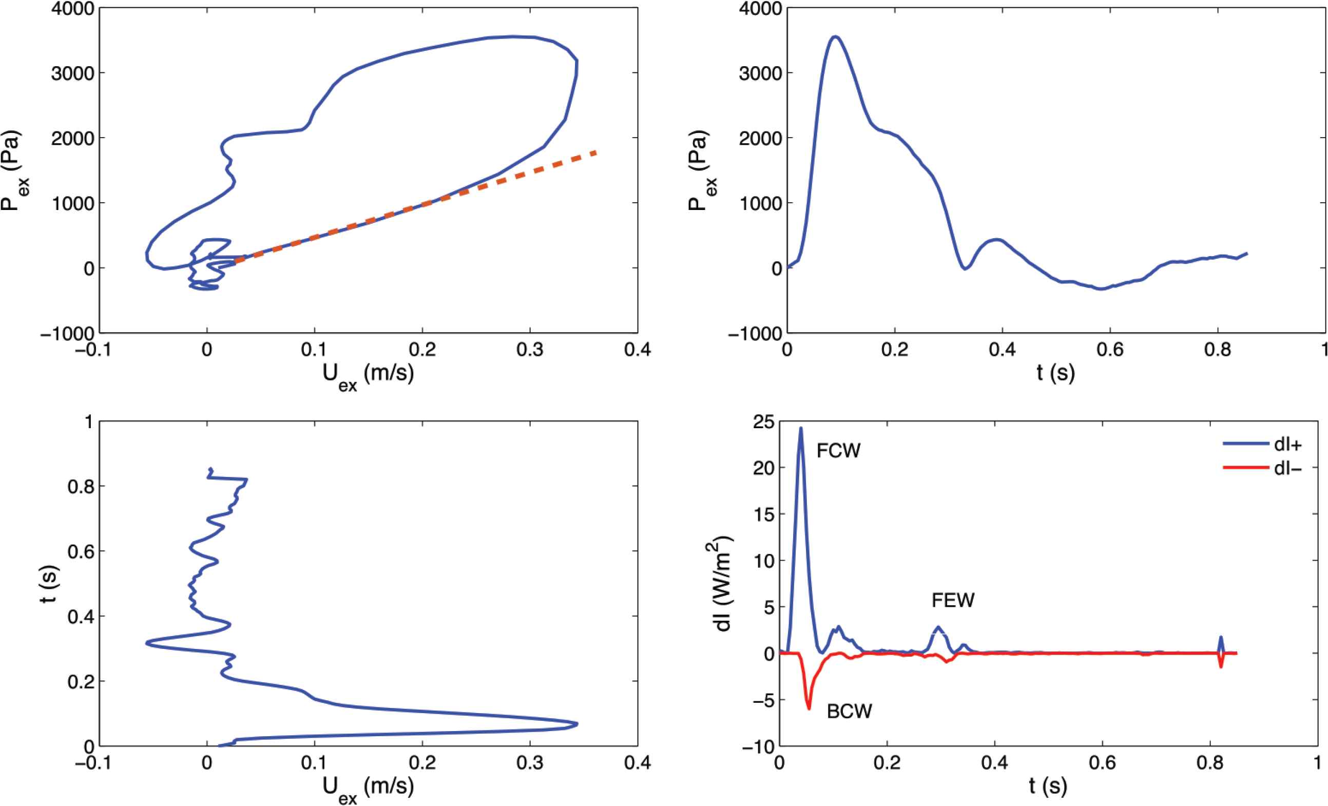
Example of PexUex loop (Top left), Pex contour (Top right), Uex contour (Bottom left) and corresponding wave intensity [Bottom left; see Equation (5)] for one subject. A straight line highlighting the slope of the linear portion is superimposed on the PexUex loop [see Equation (4)]. Forward Compression Wave (FCW), Backward Compression Wave (BCW) and Forward Expansion Wave (FEW) are labelled in the wave intensity plot. dI+, forward wave intensity component; dI−, backward wave intensity component.
After the calculation of wave speed and wave intensity, relevant wave intensity parameters were extracted. The area (J/m2) of the Forward Compression Wave (FCW), generated by the contraction of the left ventricle, was calculated from the area of the early-systolic peak observed in dI+ (Figure 3). Similarly, the area of the Backward Compression Wave (BCW), which is attributed to reflections from the head microcirculation if it is measured in the common carotid artery, was determined from the area, of the mid-systolic peak present in dI−. Finally, the area of the Forward Expansion Wave (FEW), which is generated by the decrease in shortening velocity of the left ventricle in late systole, was determined from the area of the late-systolic peak seen in dI+.
2.7. Statistical Analysis
All values are reported as mean ± SD, relative to the whole cohort, in the text, tables and figures. SPSS Statistics (version 20, IBM, Armonk, NY, USA) was used to design the statistical analysis. Hemodynamic and wave intensity parameters were compared via one-way analysis of variance followed by Tukey’s post-hoc. Significance threshold was set at adjusted p = 0.05.
3. RESULTS
All changes are referred to the reference value for that particular parameter (as detailed in Table 2).
Pex max (Figure 4) did not significantly change with negative P∞ variations (−25%, −50%, −75%) but decreased significantly with respect to the reference value (w.r.t.R) with positive P∞ variations, up to +50%; then it increased again. The biggest change w.r.t.R was at +50% variation and its amplitude was −12% (p < 0.05). SD did not substantially change with P∞ variations.
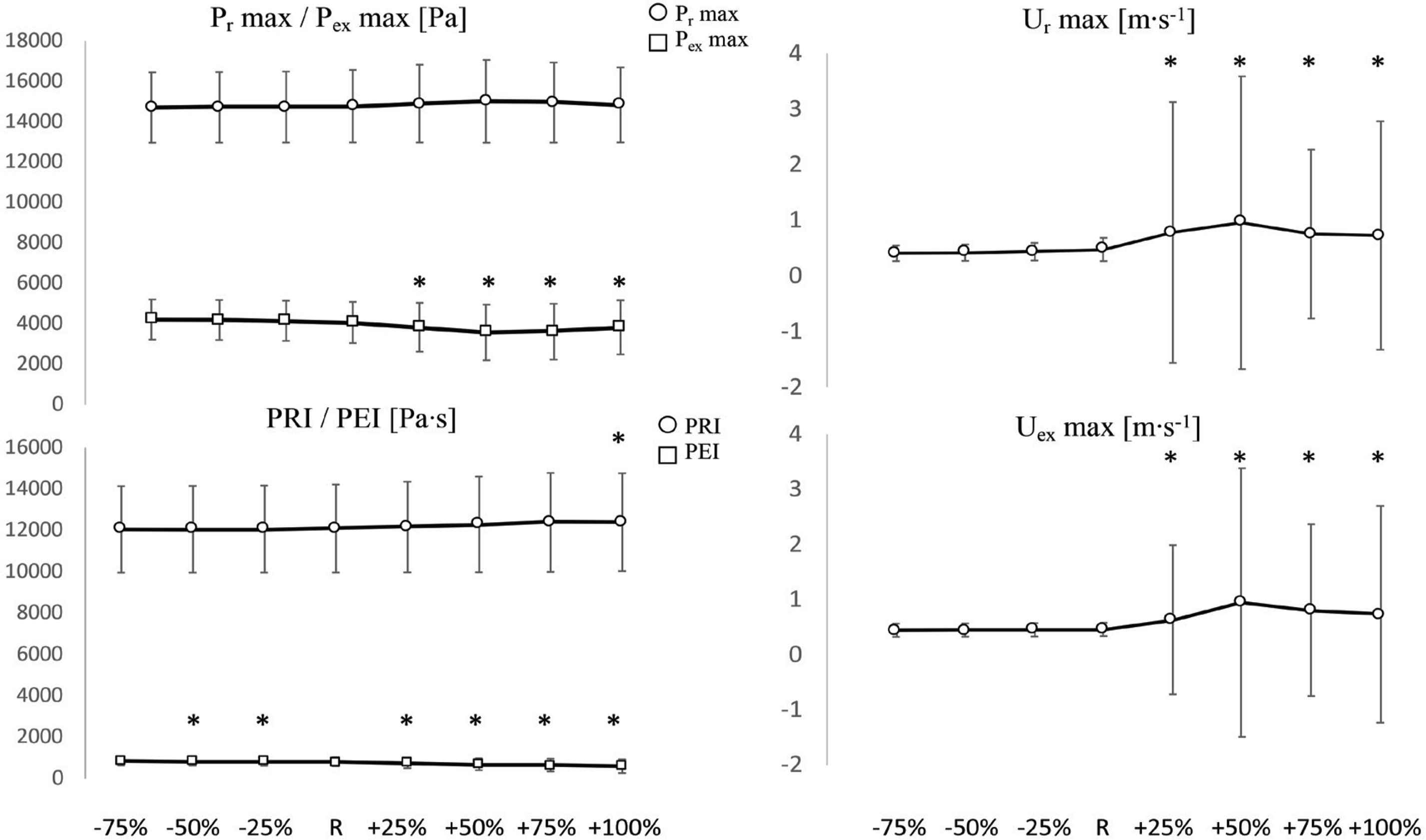
Comparisons of Pr max and Pex max (Top left), Ur max (Top right), PRI and PEI (Bottom left) and Uex max (Bottom right) values among positive (+25%, +50%, +75%, +100%) and negative (−25%, −50%, −75%) variations of P∞, with respect to the reference value (R). *Significant difference with respect to R (p < 0.05). Y-axis units are reported in each figure title. Values are reported as mean ± SD (n = 1037).
Pr max (Figure 4) did not significantly change: it had a tendency to decrease w.r.t.R with negative P∞ variations and to increase with positive P∞ variations, up to +50%. The maximum change w.r.t.R was recorded at +50% and its amplitude was +1.6% (p > 0.05). SD did not substantially change with P∞ variations.
PEI (Figure 4) decreased (significantly w.r.t.R) with positive P∞ variations and slightly increased (significantly w.r.t.R, except at −75%) with negative P∞ variations. The biggest changes w.r.t.R were: −26% (p < 0.05) at the biggest positive variation (+100%) and +5% (p < 0.05) at the opposite side (−75% variation). PRI (Figure 4) had a tendency to decrease with negative P∞ variations and to increase with positive variations. Overall, its value did not substantially change: the maximum increase was at +100% variation and its corresponding amplitude was +3% (p < 0.05). SD did not substantially change for both PEI and PRI.
Ur max and Uex max (Figure 4) had very high SD at positive P∞ variations. Ur max did not significantly change w.r.t.R with negative P∞ variations but had a tendency to decrease (maximum change: −14% at −75% variation) whereas it significantly increased w.r.t.R with positive P∞ variations (maximum change: +100% at +50% variation). At +75% and +100% iterations, it had a tendency to decrease again. The same behaviour applied to Uex max: the maximum changes had amplitudes of +106% at +50% variation and −3% at −75% variation, respectively. The increases in the positive direction were significant whereas all decreases in the negative direction were non-significant.
The diastolic constant b (Figure 5) did not change significantly w.r.t.R, with all negative P∞ variations, but had a tendency to decrease, whereas it increased (significantly w.r.t.R) with positive P∞ variations, up to +75%. The SD substantially increased with positive variations. The systolic constant a (Figure 5) had also a tendency to decrease (non-significantly w.r.t.R) with negative P∞ variations whereas significantly increased with all positive P∞ variations, up to +50%, resembling the behaviour of b.

Comparisons of rate constant a (Left) and diastolic rate constant b (Right), among positive (+25%, +50%, +75%, +100%) and negative (−25%, −50%, −75%) variations of P∞, with respect to the reference value (R). *Significant difference with respect to R (p < 0.05). Y-axis units are reported in each figure title. Values are reported as mean ± SD (n = 1037).
Wave speed (Figure 6) did not substantially change: it slightly increased (non-significantly w.r.t.R) with negative P∞ variations (maximum change: +2% at −75% iteration) and tended to decrease (non-significantly w.r.t.R) with positive P∞ variations (maximum change: −7% at +75% iteration). SD tended to remain stable.
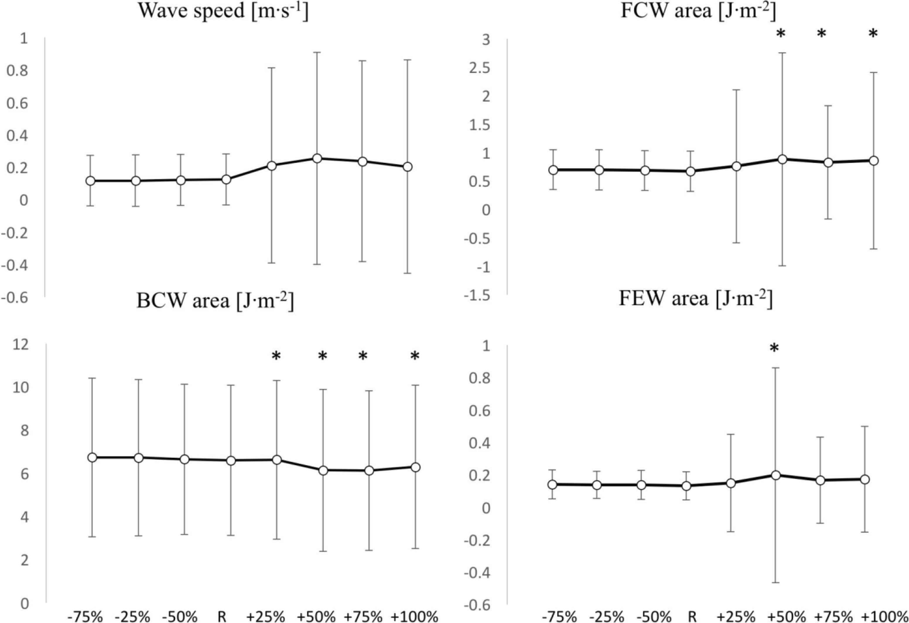
Comparisons of wave speed c (Top left), FCW area (Top right), BCW area (Bottom left) and FEW area (Bottom right) values among positive (+25%, +50%, +75%, +100%) and negative (−25%, −50%, −75%) variations of P∞, with respect to the reference value (R). *Significant difference with respect to R (p < 0.05). Y-axis units are reported in each figure title. Values are reported as mean ± SD (n = 1037).
In the context of wave intensity analysis, FCW area (Figure 6) increased with positive variations (significantly w.r.t.R, except for +25% iteration) whereas it remained unchanged with negative variations. Maximum changes were +32% at +50% variation in the positive direction and +4% (p > 0.05) at −75% variation in the negative direction. FEW area (Figure 6) had a tendency to increase in both directions of variation, although its increases were all non-significant, except for the +50% iteration. Maximum changes were +49% at +50% variation in the positive direction and +7% at −75% variation in the negative direction. SD tended to increase in the positive direction and to remain stable in the negative direction, for both FCW and FEW areas.
Finally, BCW area (Figure 6) significantly increased in the positive direction and non-significantly changed in the negative direction. The maximum changes were: −7% (p > 0.05) at −75% variation and +103% at +50% variation.
4. DISCUSSION
The concept of reservoir pressure has already been used in research and clinical studies, we believe it is crucially important to establish the effect of the value of P∞ on the determination of wave speed and wave intensity analysis, which are being used to characterise arterial stiffness and cardio-arterial interaction, respectively. We determined P∞ by fitting the diastolic pressure decay as described earlier [3], calculated wave speed using the PU-loop (Pressure-Velocity Loop) [12] and carried out wave intensity analysis [13]. We varied the value of P∞ from −75% to +100% and calculated the corresponding values of hemodynamic parameters.
The concerns pertaining the validity of the reservoir-wave approach continues [14,15] and the suitability of the technique is hotly debated both in the research and clinical fields [16–18]. However, the scope of this parametric study was to assess the sensitivity of the derived parameters as a function of the value of the asymptotic pressure. Further, the suitability of using a single exponential function to model the diastolic decay is also questioned by the recent work of Parker [15], who suggested that multi-exponential models might be more appropriate to describe the pressure waveform in diastole, reflecting the behaviour of many high-order modes of the waves. In this study, however, we chose to model the pressure decay with a single exponential and a single asymptotic value to allow direct comparisons with previous work.
The analysis in the present study was performed on clinical vascular data of a middle aged healthy human cohort. Hemodynamic and wave intensity parameters were compared using different P∞ values in the fitting of the reservoir pressure and velocity waveforms, assuming the reservoir-wave hypothesis for the decomposition of the measured arterial pressure.
Wave intensity analysis requires value of wave speed for the determination of the forward and backward wave intensities. Wave speed in this study was determined using the PU-loop method [Equation (4)], which assumes the absence of reflected waves during the early part of systole, and that waves are unidirectional. Although Segers et al. [19] questioned this assumption regarding the loop techniques and found that PU-loop method may lead to an overestimation of wave speed in the carotid artery, Borlotti et al. [11] and Pomella et al. [20,21] have successfully used the lnDU-loop (Diameter-Velocity loop) technique also in the carotid artery with the later studies carried out during exercise. While we acknowledge the possible existence of reflected waves in the carotid artery in early systole, we do not consider this to be relevant to the scope of this study and should not impact the results or the conclusions related to the reservoir-wave approach.
Table 2 reports the actual P∞ values used in this analysis. It emerged that asymptotical pressure values smaller than the used reference (48.6 ± 21.0 mmHg) did not bring substantial changes to hemodynamic and wave intensity parameters, whereas greater values brought significant “unrealistic” changes to almost all hemodynamic and wave intensity parameters, as demonstrated by the high standard deviations involved. However, these unrealistic changes were not observed in the reservoir pressure features, such as Pr max and PRI. Overestimation of P∞ did not induce unrealistic values of wave speed either. Hence, reservoir pressure and wave speed, being substantially independent of the fitting parameter, could be used as reliable diagnostic indicators.
It is also important to emphasize that the reference value of P∞ is inevitably cohort-dependent, but considering the width of the range of pressure values for which significant changes in the analysed physiological features could not be seen, we can confidently state that 12.2 < P∞ < 48.6 mmHg would be a safe range to work with. This is in line with results of Hughes et al. [22], who performed a meta-analysis of asymptotic and mean circulatory filling pressure values in humans and other mammalians, for which cessation of blood flow was involved, and found a mean P∞ value of 26.5 mmHg.
4.1. Limitations
Pressure and velocity measurements were not taken simultaneously, but sequentially, as explained in the Methods section. However, the time interval between the pressure and velocity recordings was short [11], and rapid physiological perturbations were not involved in this study. Therefore, it can be safely assumed that the hemodynamic parameters did not change significantly between recordings and the sequential recordings of the data did not impact the analysis, results or conclusions negatively.
5. CONCLUSION
It is vitally important to use the correct analysis of the reservoir pressure to obtain an accurate value of the asymptotic diastolic pressure decay (P∞). Underestimation of P∞ (up to −75%) w.r.t.R does not result in substantial changes to the hemodynamic and wave intensity parameters. Oppositely, overestimation (greater than +25%) of P∞ resulted in unrealistic increases of the studied parameters and induced large standard deviations.
The reservoir pressure and wave speed determined in this study are insensitive to a wide range of −75% to +100% changes of P∞. As such, the reservoir pressure and wave speed are independent of changes to P∞ and could be more reliable diagnostic indicators compared to other parameters that are sensitive to changes in P∞ such as wave intensity analysis parameters.
CONFLICTS OF INTEREST
The authors declare they have no conflicts of interest.
AUTHORS’ CONTRIBUTION
AWK study concept and design. NP formal data analysis. EER data acquisition. NP and AWK manuscript drafting and development. AWK and PS data interpretation and manuscript editing. NP, EER, PS and AWK proofreading and editing final draft.
FUNDING
Fund for Scientific Research Flanders - FWO G.0427.03.
Footnotes
REFERENCES
Cite this article
TY  - JOUR
AU  - N. Pomella
AU  - E.R. Rietzschel
AU  - P. Segers
AU  - Ashraf W. Khir
PY  - 2020
DA  - 2020/06/15
TI  - Implications of Changing the Asymptotic Diastolic Pressure in the Reservoir-wave Model on Wave Intensity Parameters: A Parametric Study
JO  - Artery Research
SP  - 228
EP  - 235
VL  - 26
IS  - 4
SN  - 1876-4401
UR  - https://doi.org/10.2991/artres.k.200603.003
DO  - 10.2991/artres.k.200603.003
ID  - Pomella2020
ER  -